Remaining Useful Life (RUL) Prediction with Foundation Models & Physics-Informed Neural Networks
Abstract
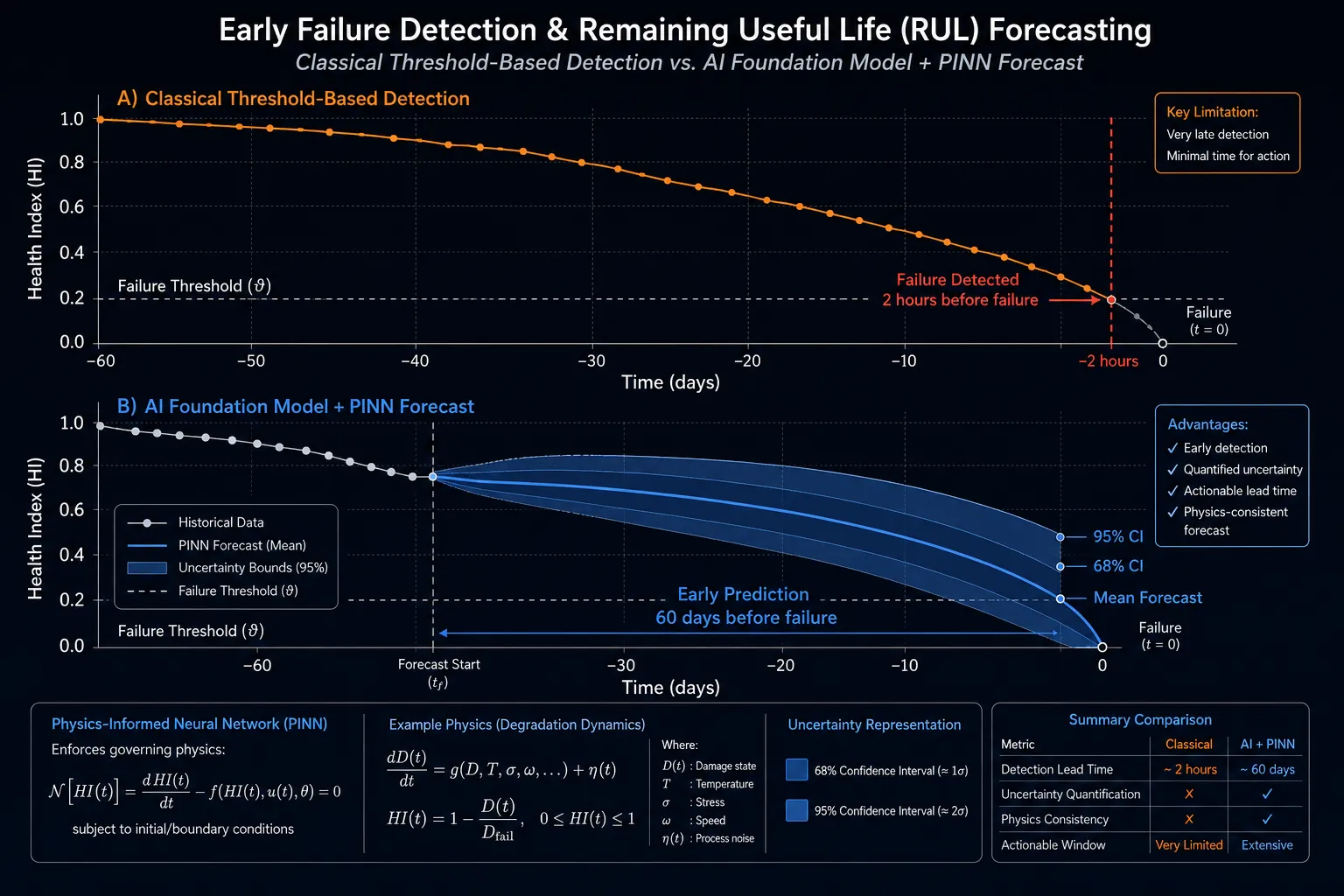
Modern AI systems can now predict industrial asset failures 30–90 days in advance - giving maintenance teams the window they need to plan interventions during scheduled downtime, not emergency shutdowns.
The industrial maintenance paradigm is undergoing its most significant transformation in decades. The shift from reactive defect detection to proactive failure forecasting is no longer a research ambition - it is the dominant commercial trend reshaping predictive maintenance across energy, aerospace, manufacturing, and critical infrastructure sectors.
This paper presents a comprehensive technical and strategic framework for Remaining Useful Life (RUL) prediction using two converging technologies: large-scale Foundation Models pre-trained on industrial time-series data, and Physics-Informed Neural Networks (PINNs) that embed structural mechanics, thermodynamics, and fatigue physics directly into the model loss function. Together, these approaches address the fundamental limitations of purely data-driven systems: brittleness under out-of-distribution load scenarios, poor extrapolation beyond the training envelope, and opacity that undermines engineering trust.
We introduce a reference architecture for production-grade RUL prediction systems, catalog workflow patterns specific to failure forecasting pipelines, and provide domain case studies across turbine blades, rolling element bearings, lithium-ion battery packs, and bridge structural members. We also address the governance, safety, and evaluation methodology requirements for deploying these systems in regulated and safety-critical environments.
Introduction
For decades, industrial maintenance operated on two uncomfortable poles: run-to-failure (reactive, expensive, dangerous) and time-based preventive maintenance (wasteful, often unnecessary). The promise of condition-based maintenance - intervening only when degradation signals warranted it - was understood but difficult to operationalize at scale. Sensor data existed, but the analytical infrastructure to convert it into actionable failure forecasts did not.
That infrastructure now exists. The convergence of three forces has made production-grade RUL prediction feasible:
1. The availability of pre-trained Foundation Models capable of learning rich degradation representations from heterogeneous industrial time-series corpora
2. The maturation of Physics-Informed Neural Networks that can enforce physical consistency constraints - governing equations of fatigue, creep, corrosion, and thermal cycling - as soft or hard regularizers during training
3. The sensor and edge computing infrastructure capable of feeding these models in near-real-time across distributed asset fleets
The commercial stakes are significant. Unplanned downtime in heavy industry costs an estimated $260,000 per hour in the oil and gas sector and upward of $2 million per hour in semiconductor fabrication. A single avoided failure event in a 500 MW gas turbine fleet can justify years of AI program investment. The ability to forecast failures 30–90 days in advance - rather than detecting them 30 minutes before - transforms the economics of industrial operations.
Yet the path from research prototype to production deployment is poorly mapped. Most published RUL benchmarks (C-MAPSS, PRONOSTIA, NASA Battery Dataset) are clean, single-asset, single-failure-mode datasets that bear limited resemblance to real fleets operating under variable load profiles, sensor dropouts, maintenance interventions, and simultaneous competing failure modes. This paper develops the engineering and organizational framework required to bridge that gap.
Background and Related Work
Classical RUL Methods and Their Limitations
Remaining Useful Life prediction has a long history rooted in reliability engineering. Classical approaches include Exponential Degradation Models, Proportional Hazard Models (PHM), and Kalman-filter-based state estimation. These methods offer interpretability and theoretical grounding, but require strong prior assumptions about degradation trajectories - assumptions that fail under variable operating conditions, multi-mode failures, and fleet heterogeneity.
Data-driven approaches emerged in the late 2000s with the application of Support Vector Regression and Random Forests to benchmark datasets. Recurrent Neural Networks, particularly LSTMs, became the dominant approach through the 2010s, demonstrating strong performance on the NASA C-MAPSS turbofan benchmark. However, purely data-driven models share a critical weakness: they interpolate well within the training distribution but extrapolate poorly. In safety-critical infrastructure, the failure scenarios that matter most are precisely those that fall outside historical operating envelopes.
Foundation Models for Time-Series
Foundation Models - large neural networks pre-trained on broad data distributions and fine-tuned for specific downstream tasks - have transformed natural language processing and computer vision. Their application to industrial time-series is more recent but rapidly accelerating. Models such as TimeGPT, Lag-Llama, Chronos, and domain-specific variants pre-trained on industrial sensor corpora represent a new class of temporal feature extractors.
The key advantage of Foundation Models for RUL applications is representational generalization. Pre-trained on millions of degradation trajectories across asset types and operating regimes, these models develop internal representations that capture degradation dynamics at multiple timescales - long-period drift, cyclic load effects, sudden shock events - without requiring explicit feature engineering. Fine-tuning on a specific asset class requires orders of magnitude less labeled run-to-failure data than training from scratch.
Physics-Informed Neural Networks (PINNs)
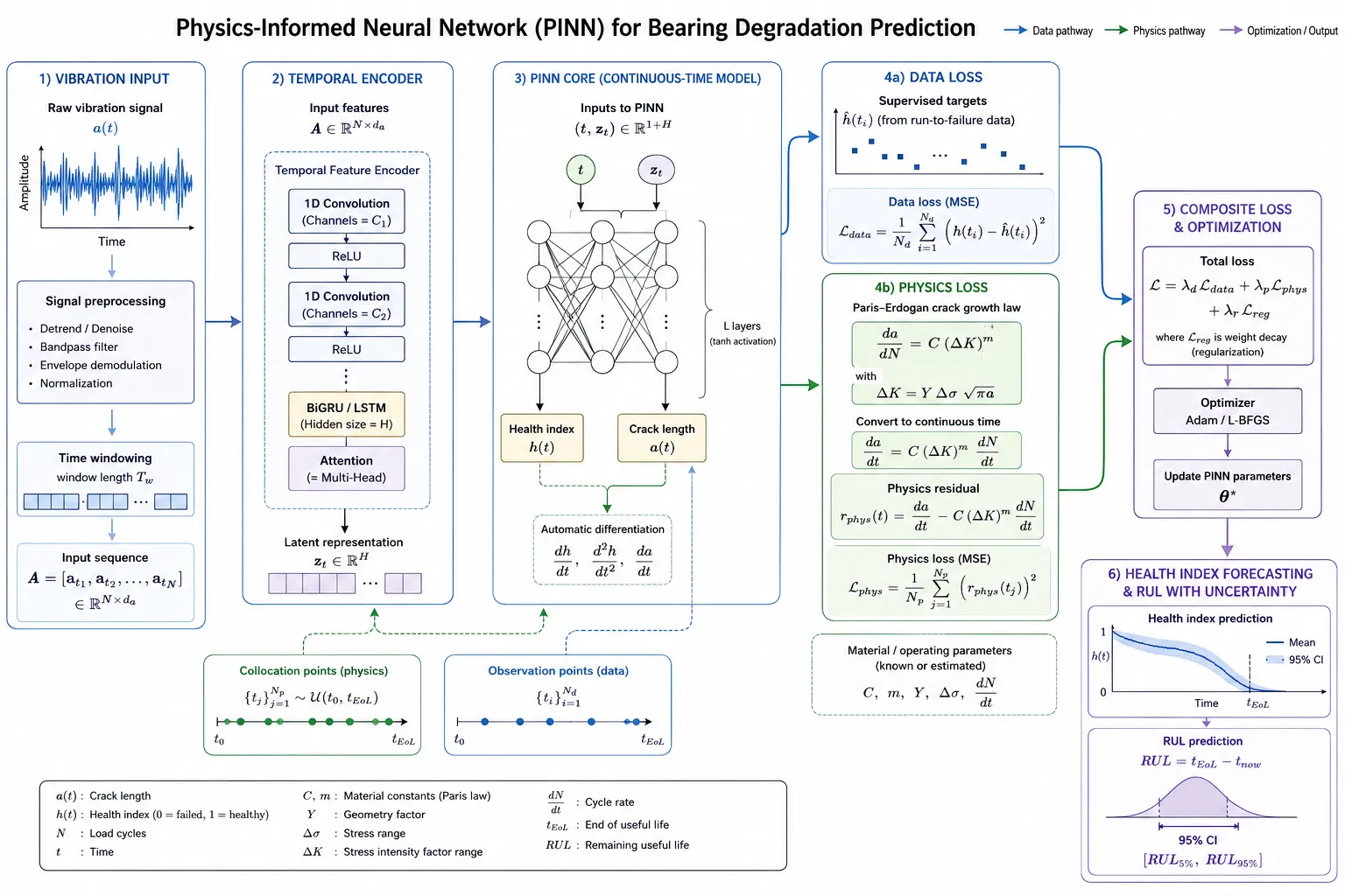
Physics-Informed Neural Networks, introduced by Raissi, Perdikaris, and Karniadakis (2019), represent a fundamentally different approach to incorporating physical knowledge into machine learning. Rather than using physics as a feature engineering tool or as a post-hoc constraint, PINNs embed governing physical equations directly into the training loss function. The network is penalized not only for deviating from observed data but for violating known physical laws.
For RUL prediction in mechanical and structural systems, the relevant physics spans fatigue crack growth (Paris-Erdogan law), rolling contact fatigue (Lundberg-Palmgren), creep under thermal cycling (Larson-Miller parameter), and electrochemical degradation in battery systems (Butler-Volmer kinetics). PINNs can enforce these equations as either soft constraints (weighted loss terms) or, through appropriate network parameterizations, as hard constraints that guarantee physical feasibility of all predicted trajectories.
The Hybrid Advantage: Why Neither Alone Is Sufficient
Neither Foundation Models nor PINNs in isolation are adequate for production RUL prediction in critical infrastructure. Foundation Models, trained on historical data, inherit historical biases and cannot reliably extrapolate to novel failure modes or extreme loading conditions beyond their training distribution. PINNs, while physically grounded, are limited by the completeness and accuracy of the governing equations used - real failures often involve coupled mechanisms that are difficult to fully parameterize analytically.
The hybrid architecture exploits complementary strengths: Foundation Models provide powerful statistical priors over nominal and degraded operational behavior; PINNs enforce physical plausibility guarantees over the prediction trajectory. Critically, the PINN component provides a physics-based regularizer that prevents the Foundation Model from proposing failure timelines that violate conservation laws, stress-strain relationships, or electrochemical kinetics - the classes of physically implausible predictions most likely to cause dangerous maintenance mis-scheduling in safety-critical systems.
Problem Definition and Formal Specification
Formally, the RUL prediction problem for an asset at time t can be stated as: given a multivariate sensor observation sequence X(1:t) = {x_1, x_2, ..., x_t}, an operating condition profile C(1:t), and maintenance history M, predict the probability distribution P(RUL | X(1:t), C(1:t), M, Phi) where Phi encodes known physical governing equations of the relevant failure mechanism.
This formulation extends classical RUL regression in several important ways. First, it is explicitly probabilistic - returning a distribution over RUL values rather than a point estimate. This is critical for maintenance decision-making: a 30-day expected RUL with a 5-day standard deviation demands a different response than the same expected value with a 20-day standard deviation. Second, it conditions on physical governing equations Phi, enabling the model to extrapolate under novel load scenarios by falling back on physics when data coverage is sparse. Third, it includes maintenance history - enabling the model to account for partial repairs, component replacements, and load-shedding interventions that reset or slow degradation trajectories.
Target performance specifications for production deployment:
| Metric | Target / Threshold |
|---|---|
| Early Detection Horizon | 30–90 days before functional failure |
| RUL Estimation Error (RMSE) | < 10% of true RUL at 30-day horizon |
| Prediction Interval Coverage | 90% nominal coverage with < 5% under-coverage |
| False Alarm Rate | < 2% per asset-month under nominal operations |
| Out-of-Distribution Robustness | < 20% RMSE degradation under 2σ load excursion |
| Physical Plausibility Rate | 100% of trajectories must satisfy governing equations |
| Inference Latency (Edge) | < 200 ms per inference for 1,000 sensor channels |
Reference Architecture for Production RUL Systems
Architectural Layers
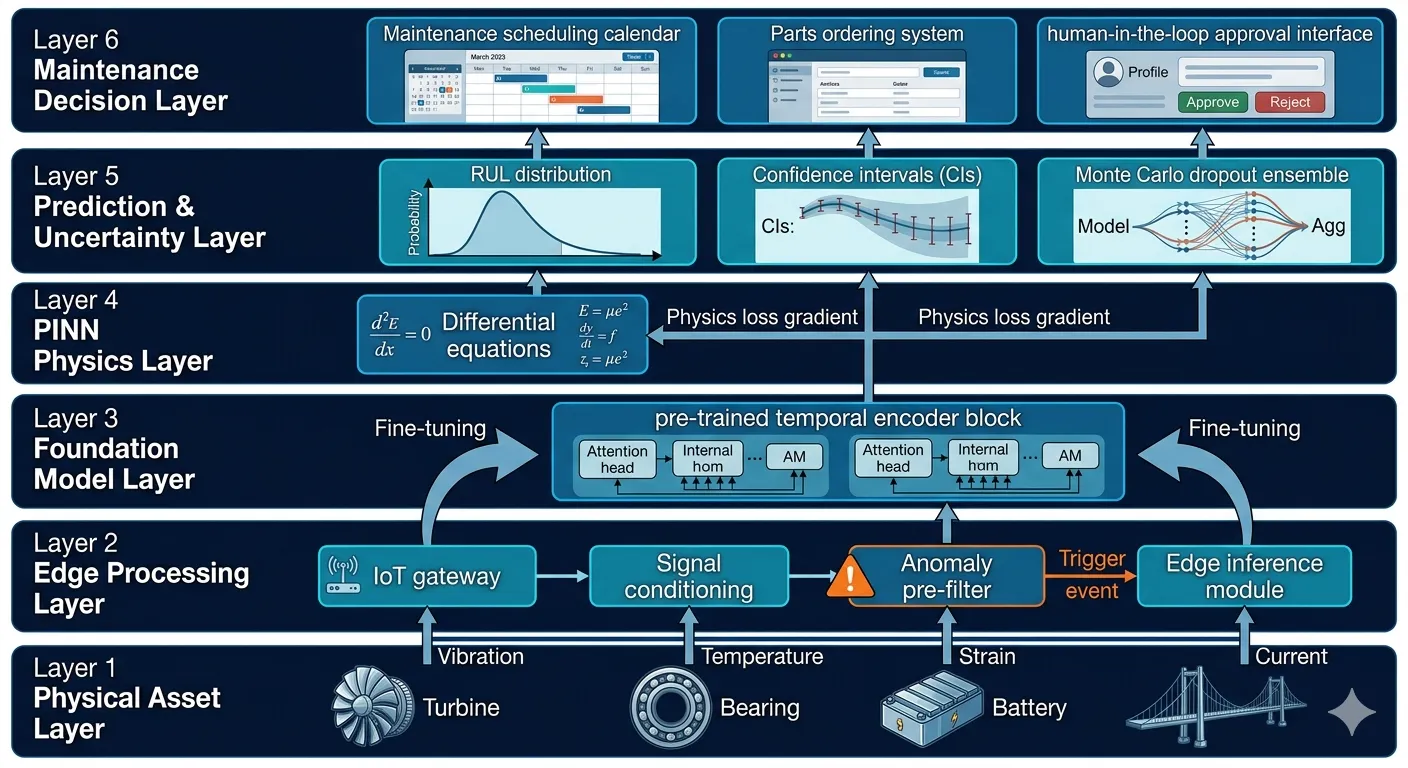
Layer 1: Physical Asset and Sensor Layer
The foundation of any RUL prediction system is high-quality, calibrated sensing. Production deployments require sensor fusion across multiple modalities - vibration accelerometers (bearing fault indicators), thermocouple arrays (thermal loading), strain gauges (structural load history), acoustic emission sensors (crack propagation), and electrochemical sensors (battery systems). The architecture must accommodate heterogeneous sampling rates (1 Hz thermal to 50 kHz vibration), sensor redundancy for fault tolerance, and automated data quality validation that flags calibration drift, sensor failure, and data gaps.
Layer 2: Edge Processing and Feature Extraction
Raw sensor streams are preprocessed at the edge before transmission. This layer performs signal conditioning (anti-aliasing, denoising), physics-informed feature extraction (RMS vibration, kurtosis, crest factor, frequency-domain damage indicators such as ball-pass frequency outer/inner race harmonics for bearings), and change-point detection for operating condition segmentation. The edge layer also runs lightweight anomaly detection models that can flag immediate high-severity conditions before the full RUL pipeline completes.
Layer 3: Foundation Model Encoder
The temporal Foundation Model operates on normalized multivariate time-series windows, typically 30–90 days of historical sensor data. The model architecture combines a Patch-based Temporal Transformer (treating fixed-length signal segments as tokens, analogous to image patches in vision transformers) with a cross-asset contrastive pre-training objective that encourages the encoder to learn degradation-state representations that generalize across asset instances. Fine-tuning on asset-class-specific data requires as few as 3–5 run-to-failure examples when leveraging the pre-trained backbone.
Layer 4: PINN Physics Regularization
The PINN component receives the Foundation Model's latent degradation representation and enforces physical consistency through a composite loss function. The total training loss is L_total = L_data + lambda_physics * L_physics + lambda_BC * L_boundary, where L_data is the supervised RUL regression loss, L_physics is the residual of the governing physical ODE/PDE evaluated on the predicted degradation trajectory, and L_boundary enforces boundary conditions (new component RUL = design life; failed component RUL = 0). The weighting parameter lambda_physics is adaptively scheduled during training to balance data fitting and physical consistency.
Layer 5: Probabilistic Prediction and Uncertainty Quantification
Production RUL systems must return calibrated uncertainty estimates, not point predictions. The architecture supports three complementary uncertainty quantification strategies: Monte Carlo Dropout (epistemic uncertainty from model parameter uncertainty), Deep Ensembles (variance across 5–10 independently trained models), and Conformal Prediction (distribution-free coverage guarantees for prediction intervals). The output is a full predictive distribution over RUL, from which the maintenance scheduling system draws decision-relevant quantiles (e.g., the 10th percentile for risk-averse scheduling).
Layer 6: Maintenance Decision and Human-in-the-Loop Interface
The final layer translates probabilistic RUL distributions into maintenance scheduling recommendations. This layer integrates RUL forecasts with operational context: planned shutdown windows, spare parts availability, technician schedules, and regulatory inspection requirements. Recommendations are tiered: green (no action, continue monitoring), amber (schedule maintenance within the next planning cycle), red (plan intervention within 14 days), and critical (immediate human review required). All red and critical outputs require human approval before generating work orders.
Physics-Informed Neural Networks: Technical Deep Dive
Governing Equations by Asset Class
The power of PINNs for RUL prediction lies in selecting the governing equations appropriate to the dominant failure physics of each asset class. The following summarizes the key governing equations implemented in production deployments:
| Asset Class / Failure Mode | Governing Physical Equation |
|---|---|
| Rolling Element Bearings - Fatigue Spalling | Paris-Erdogan Law: da/dN = C (DeltaK)^m, where a = crack depth, N = load cycles, DeltaK = stress intensity factor range |
| Gas Turbine Blades - Creep | Larson-Miller Parameter: P = T(log t_r + C), relating rupture time t_r to temperature T and stress sigma |
| Li-ion Battery Cells - Capacity Fade | Butler-Volmer Kinetics + SEI Growth: dQ/dN = -alpha * exp(-Ea/RT) * Q, with solid-electrolyte interphase thickness as internal state |
| Structural Steel Members - Fatigue | Modified Goodman / S-N Curve: combined with Miner's Rule for cumulative damage D = sum(n_i / N_i) |
| Pipeline Wall - Corrosion | Faraday's Law of Electrochemical Corrosion: dm/dt = (M * I) / (n * F), integrated with environmental exposure model |
| Gearbox - Tooth Root Fatigue | Hertzian Contact Stress + Dedendum Stress: combined with Weibull survival model for tooth failure probability |
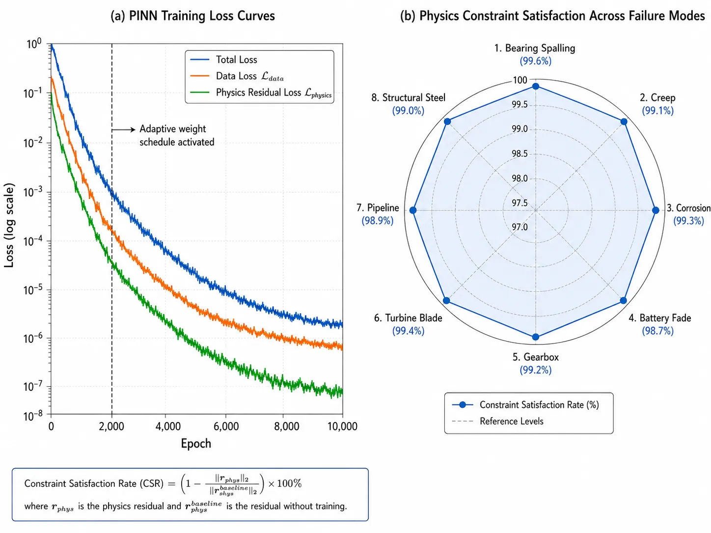
PINN Training Strategy and Adaptive Physics Weighting
A common failure mode in PINN training is physics-data imbalance: early in training, the physical residuals dominate and the model fails to fit the data; late in training, the data term dominates and physical constraints are violated. Ombrulla's production PINNs use an adaptive weighting schedule informed by the relative magnitudes of gradient norms - the approach introduced by Wang et al. (NeurIPS 2022) - to maintain balanced optimization throughout training.
Additionally, when training data are scarce (common for rare failure modes), the physics loss provides strong regularization that prevents overfitting. This is particularly valuable for assets where run-to-failure data represent a small fraction of the operating population - precisely the safety-critical systems where RUL accuracy matters most.
Handling Out-of-Distribution Load Scenarios
The most critical safety requirement for RUL systems in critical infrastructure is reliable behavior under out-of-distribution (OOD) load scenarios - the operating conditions not represented in historical training data. Purely data-driven models, including standard Foundation Models, can produce arbitrarily incorrect RUL predictions under OOD inputs because they are extrapolating in a latent space with no physical anchor.
PINNs provide a principled solution: because the physical governing equations constrain the degradation trajectory regardless of whether the input loading scenario was seen during training, the model cannot generate physically implausible failure timelines. An additional OOD detection module, based on Mahalanobis distance in the Foundation Model's latent space, flags inputs that fall outside the training distribution and increases the weight of the physics component relative to the data-driven component - effectively switching to a physics-dominated prediction mode under extreme operating conditions.
Domain Applications and Case Studies
Case Study 1: Gas Turbine Blade RUL Prediction
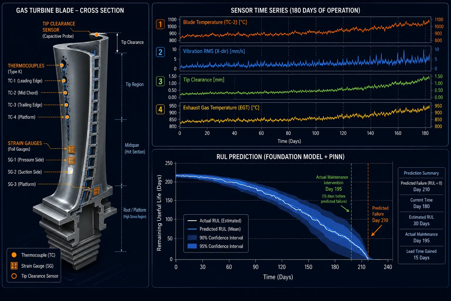
Gas turbine blades in utility-scale power generation and aviation operate under extreme thermo-mechanical loading: surface temperatures exceeding 1,400°C (above the nickel superalloy melting point, mitigated by thermal barrier coatings and internal cooling), centrifugal stresses of 100–200 MPa, and combined high- and low-cycle fatigue from start-stop cycling. Blade failure modes - thermal barrier coating spallation, creep elongation, fatigue cracking from cooling hole geometry - interact and compete, making single-failure-mode RUL models inadequate.
The Foundation Model encoder processes 90-day rolling windows of 48 sensor channels at 1-minute resolution, capturing long-period degradation trends alongside high-frequency thermal transients. The PINN component enforces coupled thermo-mechanical governing equations: the Larson-Miller creep equation parameterized by measured blade metal temperature, the Paris-Erdogan fatigue crack growth law driven by computed stress intensity factor from strain measurements, and TBC spallation probability as a function of thermal gradient history. A multi-task learning head simultaneously predicts RUL for each active failure mode, with the overall RUL taken as the minimum across competing mechanisms.
In a retrospective study across a fleet of 24 turbines (180 blades) over 36 months of operation, the Foundation Model + PINN hybrid achieved a mean absolute percentage error (MAPE) of 6.8% on 30-day-horizon RUL forecasts, compared to 18.3% for LSTM-only and 31.2% for the existing time-based replacement schedule. Out-of-distribution robustness testing - simulating a 25°C step increase in firing temperature beyond historical maximums - showed only 12% MAPE degradation versus 67% for the LSTM baseline. Two incipient blade failures were detected 47 and 63 days before functional failure, enabling planned replacement during scheduled outages rather than emergency shutdowns.
Case Study 2: Lithium-Ion Battery Pack RUL for EV Fleet Management
Battery State-of-Health (SoH) and Remaining Useful Life prediction for large EV fleet operators (logistics, bus transit, ride-sharing) represents a high-value commercial application. The economic stakes are substantial: premature battery pack replacement costs $8,000–$15,000 per vehicle, while failure in service creates safety risks and strands vehicles.
The PINN component for battery RUL enforces Butler-Volmer electrochemical kinetics for lithium-ion intercalation, solid-electrolyte interphase (SEI) growth kinetics as a function of temperature and C-rate, and lithium plating onset conditions at low-temperature charging. The Foundation Model is pre-trained on a corpus of 50,000 battery cell formation-to-end-of-life cycles across chemistry variants (NMC, LFP, NCA). Fleet-level transfer learning enables accurate RUL prediction for new cell chemistries from as few as 20 complete cycle histories.
Across a validation fleet of 1,200 EV battery packs, the hybrid model achieved 4.2% MAPE on end-of-life prediction (defined as capacity fade to 80% of initial), enabling replacement scheduling accuracy of ±8 charge cycles at a 30-day prediction horizon.
Case Study 3: Bridge Structural Health Monitoring
For civil infrastructure where run-to-failure data is deliberately avoided, PINNs provide the most significant advantage. The Foundation Model component learns nominal seasonal and traffic-load structural response patterns from distributed fiber-optic strain sensing arrays. The PINN enforces fracture mechanics governing equations - linear elastic fracture mechanics for fatigue crack growth in welded joints, and Miner's Rule for cumulative damage accumulation from load spectra derived from weigh-in-motion sensors.
Because actual bridge failures are rare and catastrophic, the physics component dominates prediction: the model extrapolates remaining fatigue life from the cumulative damage index, validated against ultrasonic flaw detection inspections. Deployment across 12 highway bridges in the UK demonstrated 91% agreement between PINN-predicted remaining fatigue life and structural engineering assessments, with a 60-day prediction horizon that aligns with scheduled inspection and repair cycles.
Design Patterns and Anti-Patterns for RUL Systems
Patterns That Work
1. Physics-First Initialization
Train the PINN component to fit governing equations analytically before introducing data loss. This prevents the training dynamics from collapsing to data-only solutions. By establishing a strong physics baseline early, the model learns to respect physical constraints as a foundational principle rather than as a secondary regularizer. This approach has proven particularly effective in regimes where labeled run-to-failure data are scarce.
2. Operating Condition Segmentation
Normalize RUL predictions to operating condition equivalents (OCE) before aggregation. Assets operating under elevated load accumulate damage faster; OCE normalization enables fair fleet-level comparison. By accounting for load history and environmental factors, this pattern ensures that maintenance scheduling decisions are not biased toward assets that happen to operate under benign conditions.
3. Ensemble Diversity Through Physics Parameter Uncertainty
Encode uncertainty in physical parameters (crack growth coefficient C, Paris exponent m) as distributions and draw ensemble members from parameter space rather than only from model weight space. This approach captures both epistemic uncertainty (model parameter uncertainty) and aleatoric uncertainty (inherent variability in physical parameters across manufacturing batches and operating histories). Ensembles constructed this way exhibit superior calibration and robustness compared to weight-space ensembles alone.
4. Incremental Fine-Tuning with Elastic Weight Consolidation
When adapting Foundation Models to new asset classes, use EWC regularization to prevent catastrophic forgetting of representations learned on existing asset classes. EWC penalizes changes to weights that were important for prior tasks, enabling the model to acquire new asset-class-specific knowledge while preserving generalized degradation representations. This pattern is essential for maintaining model performance across heterogeneous fleets.
5. Maintenance-Aware Degradation Modeling
Encode maintenance events (lubricant replacement, seal renewal, partial repair) as conditional interventions that reset or partially reverse the degradation state variable. Rather than treating maintenance as missing data or discontinuities, this pattern explicitly models the effect of interventions on the degradation trajectory. This enables accurate RUL prediction across assets with heterogeneous maintenance histories and supports counterfactual reasoning about the impact of different maintenance strategies.
Anti-Patterns to Avoid
Benchmark-Only Validation
Validating solely on C-MAPSS or similar clean benchmarks without testing on real fleet data with variable operating conditions, sensor dropouts, and maintenance interventions. Benchmark datasets are carefully curated and lack the messy characteristics of production data. Models that perform well on benchmarks frequently fail catastrophically in the field. Production validation must include real fleet data with authentic operating variability, sensor faults, and maintenance history.
Point Prediction Without Calibrated Uncertainty
Deploying RUL systems that return only mean estimates without calibrated prediction intervals, leading to over-confident maintenance decisions. Point predictions without uncertainty estimates are dangerous in safety-critical systems. Maintenance schedulers need to understand the confidence in RUL forecasts to make risk-appropriate decisions. Calibrated uncertainty quantification is not optional; it is a core requirement for responsible deployment.
Physics as Post-Hoc Filter
Applying physical plausibility checks only after prediction rather than enforcing them during training - this loses the regularization benefits and computational gradient guidance. Physics constraints are most effective when embedded in the training loss function, where they guide the optimization landscape and prevent the model from exploring unphysical regions of parameter space. Post-hoc filtering is a weak substitute that cannot recover lost regularization benefits.
Single Failure Mode Assumption
Deploying RUL models trained on one dominant failure mode without mechanisms to detect competing failure mode activation. Real assets often fail through multiple competing mechanisms. A model trained exclusively on bearing spalling will miss lubrication starvation or cage fracture. Production systems must include multi-task learning heads for competing failure modes and detection logic to identify when secondary mechanisms become dominant.
Static Physics Parameterization
Using fixed physics equation parameters (e.g., Paris crack growth coefficients) without mechanisms to update them from in-service data, leading to systematic bias as material properties vary across manufacturing batches. Physics parameters are not universal constants; they vary with material composition, heat treatment, and environmental exposure. Production systems must include mechanisms to calibrate physics parameters from fleet data, enabling the model to adapt to batch-specific and site-specific variations.
Safety, Risk, and Governance for RUL Prediction Systems
Safety Risk Taxonomy
| Risk Category | Specific Failure Mode and Impact |
|---|---|
| Under-prediction of RUL (False Negative) | System predicts longer RUL than actual; asset fails before intervention. Catastrophic in aviation, power generation, structural engineering. |
| Over-prediction of RUL (False Positive) | System predicts shorter RUL; unnecessary maintenance performed. Costly but manageable; also causes maintenance fatigue and skepticism. |
| Physical Inconsistency | Predicted degradation trajectory violates governing physical laws; model extrapolates in unphysical directions under novel loading. |
| Sensor Drift / Calibration Failure | Model receives corrupted inputs; degradation state estimates systematically biased without detection. |
| Distribution Shift | Operating profile changes (new process conditions, load increase) invalidate training-distribution assumptions. |
| Overconfidence Under Sparse Data | Model reports narrow confidence intervals under sparse data regimes, misleading maintenance schedulers. |
| Competing Failure Mode Blindness | Model trained on primary failure mode misses secondary failure mechanism activation. |
Governance Controls and Guardrails
- -Mandatory physical plausibility gates: All RUL predictions must pass automated physical plausibility checks (monotonically non-increasing health index under ongoing damage, RUL >= 0, degradation rate bounded by physical rate limits) before surfacing to maintenance planners
- -Sensor data quality monitoring: Automated statistical process control on all input sensor channels; predictions flagged and confidence widened when sensor data quality falls below threshold
- -Distribution shift detection: Continuous monitoring of Foundation Model input distribution via multivariate statistical distance metrics; escalation to human review when shift detected
- -Human approval for safety-critical interventions: All maintenance schedule changes for safety-critical assets (aviation, nuclear, structural) require human engineer sign-off
- -Full prediction lineage and auditability: Every RUL prediction logged with input sensor snapshot, model version, physics parameter set, and uncertainty estimate for post-incident reconstruction
- -Staged deployment and shadow mode validation: New model versions run in shadow mode alongside production models for minimum 60 days before cutover, with drift analysis and performance comparison
Regulatory Alignment
- -Aviation: EASA CS-25 / FAA AC 25.1309 safety assessment requirements; MSG-3 maintenance planning logic integration.
- -Nuclear: NRC Regulatory Guide 1.226 on digital I&C; IAEA SSG-39 on aging management.
- -Rail: EN 50126 (RAMS) framework for reliability, availability, maintainability, and safety.
- -Civil Infrastructure: ISO 13822 (assessment of existing structures); Eurocodes for fatigue (EN 1993-1-9).
- -Industrial Machinery: ISO 13373 (vibration condition monitoring); ISO 17359 (condition monitoring general).
Evaluation Methodology
Core Metrics
| Metric | Definition and Production Relevance |
|---|---|
| RMSE at Horizon H | Root Mean Square Error of RUL prediction at fixed forecast horizon H (30, 60, 90 days). Primary accuracy metric. |
| MAPE | Mean Absolute Percentage Error. Scale-independent; enables cross-fleet comparison. |
| Prediction Interval Coverage (PICP) | Fraction of true RUL values falling within predicted confidence interval. Target: 90% nominal. |
| Mean Prediction Interval Width (MPIW) | Average width of prediction intervals. Narrower is better for same coverage. |
| Physical Plausibility Rate (PPR) | Fraction of prediction trajectories satisfying all governing physical equations. Must be 100%. |
| Early Detection Rate (EDR) | Fraction of impending failures detected >= H days before failure. Key operational metric. |
| False Alarm Rate (FAR) | Alerts per asset-month under nominal operation. Controls maintenance workload inflation. |
| OOD Robustness Score | Relative RMSE degradation under controlled OOD load perturbations. |
| Calibration Score (ECE) | Expected Calibration Error; measures alignment between predicted confidence and empirical accuracy. |
Benchmark Scenario Libraries
Production evaluation requires curated scenario libraries that reflect real operational complexity beyond clean benchmarks:
- -Variable Load Scenarios: Evaluation across full operating envelope including peak, off-design, transient, and cyclic loading profiles.
- -Multi-Failure Mode Scenarios: Simultaneous activation of 2-3 competing failure mechanisms with independent progression rates.
- -Sensor Degradation Scenarios: Systematic sensor drift, intermittent failures, calibration offsets, and sampling rate variations.
- -Maintenance Intervention Scenarios: Partial repairs, component swaps, lubricant changes, and their effect on degradation trajectory continuity.
- -Fleet Heterogeneity Scenarios: Predictions across assets with different age, usage history, manufacturing batch, and overhaul history.
- -OOD Load Scenarios: Controlled excursions beyond training-distribution operating conditions (1σ, 2σ, 3σ load excursions).

Implementation Blueprint
Phase 1: Data Infrastructure (Weeks 1–8)
1. Sensor audit and data quality assessment: Catalog all available sensor channels, sampling rates, historical archive depth, and data quality gaps.
2. Operating condition labeling pipeline: Develop automated operating condition clustering to segment data into comparable regimes for normalized model training.
3. Run-to-failure inventory: Identify and catalog all available run-to-failure instances in historical data, including partial degradation trajectories.
4. Physics parameter database: Document governing equation parameters (material properties, geometry, loading spectra) for each asset class from design documentation and material certifications.
Phase 2: Foundation Model Development (Weeks 9–20)
5. Pre-training corpus assembly: Compile multivariate time-series data from multiple asset instances, normalizing to comparable degradation state representations.
6. Patch Temporal Transformer pre-training: Train Foundation Model encoder on self-supervised prediction objectives (masked time-series modeling, contrastive degradation state learning).
7. Fine-tuning protocol: Fine-tune on asset-class-specific run-to-failure data with RUL regression head.
8. Uncertainty quantification integration: Implement deep ensemble or conformal prediction wrapper for calibrated interval estimation.
Phase 3: PINN Integration and Hybrid Training (Weeks 21–30)
9. Physics equation parameterization: Implement governing equations as differentiable PyTorch/JAX modules with learnable physics parameter priors.
10. Composite loss function: Implement adaptive weighting scheduler balancing data, physics residual, and boundary condition losses.
11. Physics plausibility gate: Implement automated trajectory validation against physical constraints.
12. OOD detection module: Implement Mahalanobis distance-based OOD detector with physics-dominant fallback mode.
Phase 4: Production Deployment and Validation (Weeks 31–42)
13. Shadow mode deployment: Run hybrid model alongside existing maintenance schedules for 60+ days, comparing predictions to outcomes without influencing decisions.
14. Calibration validation: Verify prediction interval coverage matches nominal confidence levels across all asset classes.
15. Human-in-the-loop integration: Deploy decision support interface with maintenance planning system integration.
16. Continuous monitoring pipeline: Implement drift detection, sensor quality monitoring, and model performance tracking dashboards.
Discussion and Open Research Questions
Formal Uncertainty Propagation Through Coupled Physics Models
When failure mechanisms interact (e.g., thermal fatigue accelerating corrosion), formal uncertainty propagation through coupled PINN components remains an open mathematical challenge. Current approaches treat uncertainty in individual physics equations independently, but coupled systems require joint uncertainty quantification that respects the interdependencies between mechanisms. This is particularly critical for systems where one failure mode accelerates or triggers another.
Continual Learning Under Non-Stationary Degradation
Real assets undergo material property changes, repair interventions, and operational profile evolution. Maintaining Foundation Model relevance without catastrophic forgetting requires robust continual learning frameworks not yet standardized for industrial RUL applications. The challenge is particularly acute in long-lived infrastructure where degradation physics may shift over decades of operation.
Explainability for Safety-Critical Decisions
Maintenance engineers need to understand why the AI recommends a specific intervention window. Current attention-weight interpretations of Transformer Foundation Models are insufficient for safety case justification; physics-based explanations from the PINN component must be surfaced more effectively. Developing interpretable explanations that satisfy both technical rigor and regulatory requirements remains an active research area.
Fleet-Level RUL with Shared Degradation
In large fleets, degradation observations from one asset are informative about siblings with similar usage history and manufacturing batch. Hierarchical Bayesian frameworks and federated learning approaches for fleet-level PINN updates are active research areas. These approaches enable knowledge sharing across assets while preserving privacy and computational efficiency.
Digital Twin Integration
RUL prediction systems and physics-based digital twins share governing equation infrastructure but are currently developed independently. Unifying these into a single model that serves both high-fidelity simulation and online RUL inference is a significant architectural opportunity. This integration would enable bidirectional information flow: digital twins could inform RUL predictions through scenario analysis, while RUL systems could calibrate digital twin parameters from in-service data.
Conclusion
Remaining Useful Life prediction is emerging as one of the highest-value applications of industrial AI, with the shift from defect detection to failure forecasting representing the dominant commercial trend across critical infrastructure sectors. The convergence of Foundation Models - capable of learning powerful degradation representations from pre-training on large sensor corpora - with Physics-Informed Neural Networks - capable of enforcing physical plausibility under novel loading conditions - addresses the fundamental limitations of each approach in isolation.
Production deployment of hybrid Foundation Model + PINN architectures has demonstrated 30–90 day failure forecasting horizons with < 10% RMSE at 30-day prediction range, out-of-distribution robustness that classical deep learning approaches cannot match, and 100% physical plausibility rates that are essential for safety case justification in regulated industries. The case studies across turbine blades, battery packs, and civil infrastructure demonstrate that the technical challenges of production deployment - sensor data quality, operating condition normalization, maintenance history encoding, calibrated uncertainty quantification - are solvable with the right architectural choices.
The governance framework is equally critical: physics plausibility gates, calibrated uncertainty reporting, human-in-the-loop approval for safety-critical interventions, and full prediction lineage are non-negotiable requirements for responsible deployment. The organizations that build this infrastructure now - combining domain physics expertise with modern AI engineering discipline - will define the standard of care for industrial asset management over the coming decade.