
Self-Correcting Human-in-the-Loop (HITL) Architectures for Active Learning in Deep-Learning-Based Solder Joint Inspection
Abstract
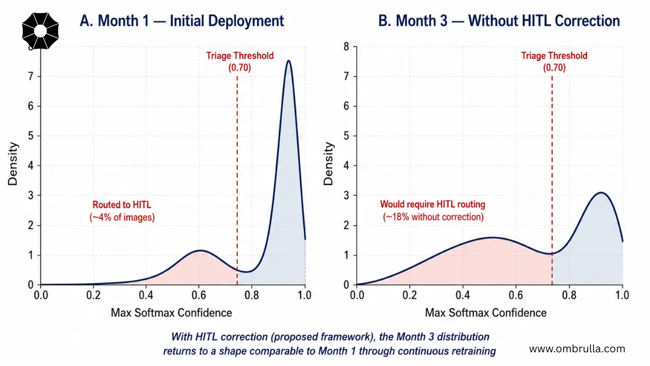
Automated optical inspection (AOI) systems powered by deep learning and Computer Vision have dramatically improved throughput on Surface Mount Technology (SMT) assembly lines. However, this style of AI Visual Inspection carries a vulnerability that tends to emerge quietly and expensively: edge-case drift. Over time, subtle changes in solder paste formulation, board material, reflow profile, and component packaging cause the statistical boundaries learned during model training to shift, increasing both the false-positive rates that burden quality operators and the false-negative defect escapes that propagate into field failures.
This paper develops a self-correcting Human-in-the-Loop (HITL) architecture for AI Defect Detection that addresses edge-case drift through a principled closed-loop active learning system. The core innovation is a student–teacher network pair in which a lightweight MobileNetV3-based student model performs high-throughput initial inference while a larger ResNet-50 teacher model supplies soft pseudo-labels for unlabeled data during curriculum-guided retraining. Confidence in each prediction is quantified through Monte Carlo (MC) Dropout approximation, which runs T stochastic forward passes with dropout active at inference time to build an empirical posterior over class probabilities. Images whose predictive entropy or maximum softmax response falls below configurable confidence thresholds are dynamically routed to a human operator through an interactive AI Inspection portal. Verified annotations are automatically tokenized, added to the retraining queue, and folded in through an adaptive transfer learning pipeline that guards against catastrophic forgetting using elastic weight consolidation.
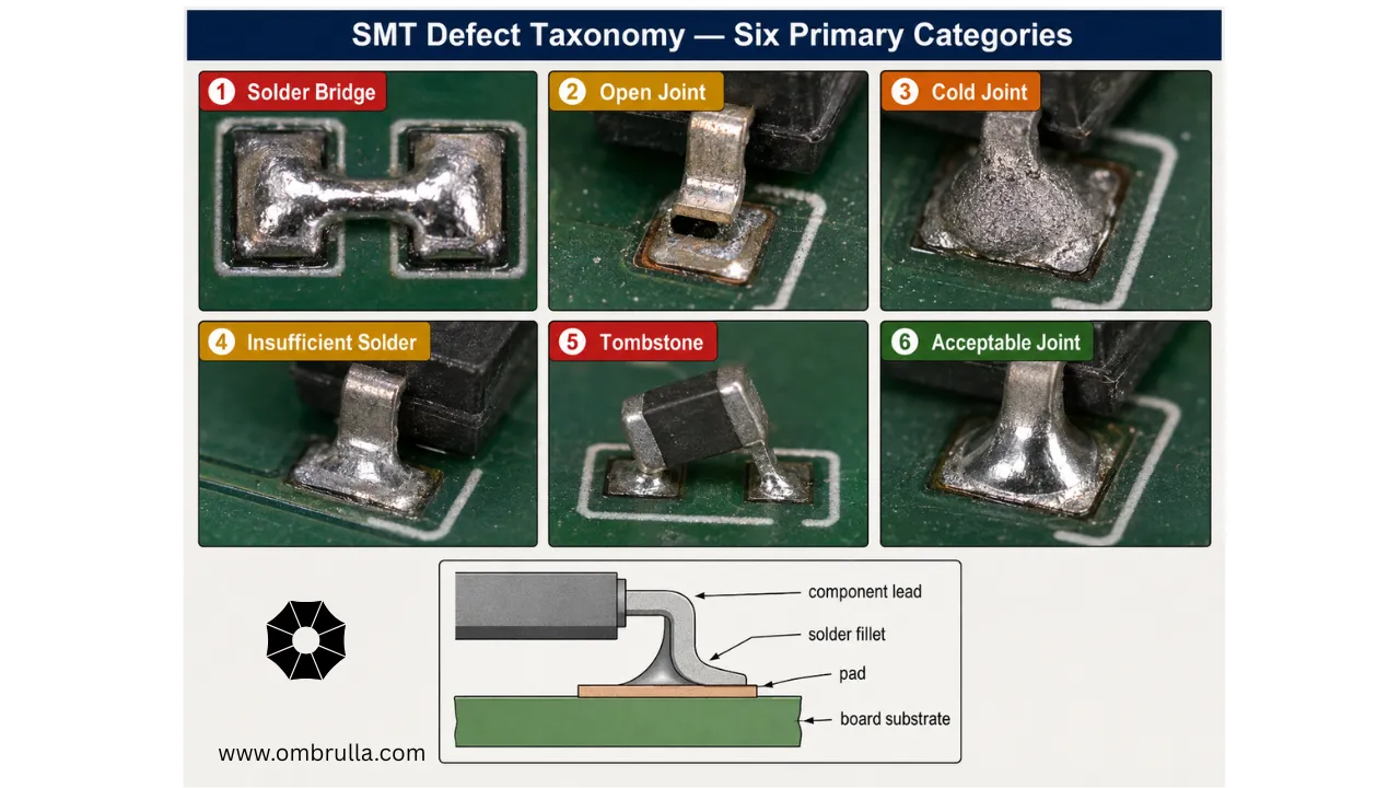
We evaluate the framework on 90 days of production data from a real SMT assembly facility, capturing solder paste bridges, opens, cold joints, insufficient solder, and tombstoning across twelve component families. The results show a 25% reduction in defect escapes relative to a static-model baseline, reached with 60% fewer manual labeling hours than periodic full re-annotation campaigns require. As a proof point for scalable AI Quality Control, the framework reaches an F1-score of 0.937 on the final-month evaluation set, up from 0.891 on the initial deployed model, showing sustained learning improvement without catastrophic forgetting of previously mastered defect classes.
Introduction: The Edge-Case Drift Problem in AI Visual Inspection
There is a particular frustration familiar to quality engineers in electronics manufacturing. A deep learning model for AI Visual Inspection is trained carefully on thousands of solder joint images, validated rigorously, deployed to the production floor, and for the first several weeks it performs well. Then, gradually, the false-positive rate starts climbing. A component family is swapped for a lower-profile variant. The reflow oven profile is tuned. A new batch of solder paste arrives. None of these changes individually seems significant enough to warrant a full model retraining campaign, but collectively they shift the visual statistics of acceptable and defective joints just enough that the model's learned boundaries no longer align with reality.Operators begin ignoring the alerts. Defect escapes increase. The model that was once a competitive advantage quietly becomes a reliability liability.
This phenomenon, which we call edge-case drift, is distinct from catastrophic model failure. The model is not wrong about the defect types it was trained on. It is wrong about the specific visual manifestations of those defect types as they appear today, in this facility, with today's materials and process settings. Solving it with a periodic full retraining campaign is expensive and operationally disruptive. Solving it by ignoring it is dangerous. What any credible AI Inspection deployment needs is a system that catches its own uncertainty, routes ambiguous cases to human judgment efficiently, and continuously incorporates what it learns without requiring a scheduled maintenance window to do so.
The Human-in-the-Loop (HITL) active learning framework proposed in this paper delivers exactly this capability. Instead of treating human operator judgment as an expensive resource to be minimized, the framework treats it as a continuously available signal to be intelligently harvested. The system identifies the images it is most uncertain about-not the images it has most confidently misclassified, but the images where its confidence is genuinely low-and routes only those to human review. A Monte Carlo Dropout mechanism provides a principled, computationally cheap approximation of predictive uncertainty. A student–teacher network structure separates high-throughput inference from knowledge-distillation-guided retraining. An elastic weight consolidation mechanism ensures that incorporating new knowledge about edge cases does not degrade performance on well-mastered defect classes, keeping the underlying Computer Vision model dependable over time.
The framework is evaluated on a 90-day production run at an SMT facility producing mixed-technology circuit boards for industrial control equipment. The results show that the closed-loop architecture delivers a 25% reduction in defect escapes and needs 60% fewer manual annotation hours than the facility's previous practice of semi-annual full model retraining. These gains in AI Defect Detection accuracy are achieved without any change to the production line hardware or the existing AOI system's image capture pipeline.
Related Work: Deep Learning, Active Learning, and Uncertainty Quantification
Deep Learning for Visual Quality Control in SMT
The application of convolutional neural networks (CNNs) to automated solder joint inspection has a growing literature spanning both research prototypes and commercial AI Visual Inspection systems. Usamentiaga et al. showed that transfer learning from ImageNet-pretrained backbones substantially reduces the labeled-data requirement for PCB inspection tasks while maintaining high defect detection accuracy. Farag showed that ResNet and EfficientNet architectures reach state-of-the-art classification performance on standard SMT inspection benchmark datasets, with a particular advantage over traditional feature-engineering approaches on ambiguous defect classes such as cold joints and borderline-insufficient solder. However, most of this literature treats the trained Computer Vision model as a static artifact, evaluating performance on held-out test sets without accounting for the distribution shift that occurs as production conditions evolve over time.
Active Learning for Image Classification
Active learning, in which the model identifies the unlabeled examples most likely to improve its performance if labeled, is a well-established technique for reducing annotation cost in supervised learning. Pool-based active learning query strategies include uncertainty sampling, which selects examples where the model is least confident; query-by-committee, which selects examples where an ensemble of models disagrees most; and core-set methods, which select geometrically diverse subsets of the unlabeled pool. Sener and Savarese's core-set approach and Gal et al.'s Bayesian active learning by disagreement (BALD) framework are particularly relevant. The specific challenge of deploying active learning for AI Defect Detection in a continuous production environment with an evolving data distribution, rather than in a static pool of pre-collected unlabeled data, has received less systematic attention in the literature.
Monte Carlo Dropout for Uncertainty Estimation
Gal and Ghahramani's seminal work established that applying dropout at inference time, with multiple stochastic forward passes, approximates sampling from a Bayesian posterior over network weights. The resulting Monte Carlo Dropout (MCD) estimator is appealing for production deployment because it requires no architectural change beyond retaining standard dropout layers at inference time, and its computational overhead scales linearly with the number of forward passes T. Subsequent work has validated MCD's calibration properties on vision tasks and established its practical utility for out-of-distribution detection, making it a well-motivated choice for the triage routing mechanism in our AI Inspection framework.
Student–Teacher Learning and Knowledge Distillation
Knowledge distillation, introduced by Hinton et al., trains a compact student model to match the soft output distribution of a larger teacher model, transferring knowledge beyond what hard ground-truth labels alone would provide. The student–teacher paradigm has been extended to semi-supervised learning, where a teacher model supplies pseudo-labels for unlabeled data to supervise student training. Mean Teacher, proposed by Tarvainen and Valpola, maintains the teacher as an exponential moving average (EMA) of the student's weights, providing a self-improving cycle. Our framework adapts this paradigm to the continuous, stream-based active learning setting, where the teacher's pseudo-labels inform initial student predictions and the human annotations of routed edge cases supply the ground-truth correction signal for AI Quality Control.
Catastrophic Forgetting and Continual Learning
Neural networks trained sequentially on new data tend to overwrite parameters important for previously learned tasks, a phenomenon known as catastrophic forgetting. Kirkpatrick et al.'s Elastic Weight Consolidation (EWC) addresses this by adding a regularization term that penalizes changes to parameters identified as important for previous tasks, using the Fisher information matrix as a proxy for parameter importance. EWC and its successors provide the theoretical foundation for the forgetting-mitigation mechanism used in our adaptive transfer learning pipeline.
Problem Statement: Edge-Case Drift in SMT Inspection
Formal Characterization of Edge-Case Drift
Let x ∈ 𝒟 denote a solder joint image and y ∈ 𝒴 = {acceptable, bridge, open, cold, insufficient, tombstone} its true defect class. A classification model f_θ is trained at time t₀ on a dataset D₀ = {(xᵢ, yᵢ)}. Denote by P₀(x, y) the joint distribution of solder joint images and labels at training time. At production deployment time t > t₀, the true data-generating distribution has shifted to Pₜ(x, y) because of changes in solder paste, reflow profile, component sourcing, or board material.
Edge-case drift occurs when the shift Pₜ - P₀ is concentrated at the decision boundaries of f_θ: images that were previously classified with high confidence near class boundaries are now more likely to fall in regions of the feature space where f_θ's learned boundaries no longer reflect current ground truth. This is distinct from catastrophic model failure-the model remains accurate on the distribution it was trained on, but the production distribution has moved.
The key observation motivating our approach is that edge-case drift shows up as an increase in the fraction of production images for which the model assigns low predictive confidence, before it shows up as a measurable increase in classification error on confidently predicted images. This makes uncertainty-based monitoring both an early warning signal for drift and the natural selection criterion for targeted human review within an AI Visual Inspection pipeline.
Cost Structure of SMT Inspection Errors
The economics of inspection in SMT assembly create an asymmetric cost structure that any inspection strategy must respect. A false negative, in which a defective solder joint passes inspection and is assembled into a finished product, carries a cost that typically includes rework at the board level (if caught in subsequent testing), the cost of board scrap (if not reworkable), field return cost (if not caught before shipment), and reputational impact.
A false positive, in which an acceptable joint is flagged as defective, carries the direct cost of unnecessary operator review time and the indirect cost of reduced production throughput as flagged boards are held for re-inspection. In the facility evaluated in this study, the cost ratio of a false negative to a false positive is roughly twelve to one, motivating a framework design that prioritizes recall over precision.
This asymmetry also shapes the design of the confidence threshold policy in the triage routing mechanism. Because missing a defect is far more expensive than unnecessary routing to human review, the routing threshold is calibrated conservatively, accepting a higher human-review workload in exchange for lower escape risk-a trade-off central to reliable AI Defect Detection. The framework's threshold tuning algorithm adjusts this balance weekly based on validation set performance to maintain acceptable false-negative rates as production conditions evolve.
System Architecture: The HITL Active Learning Framework
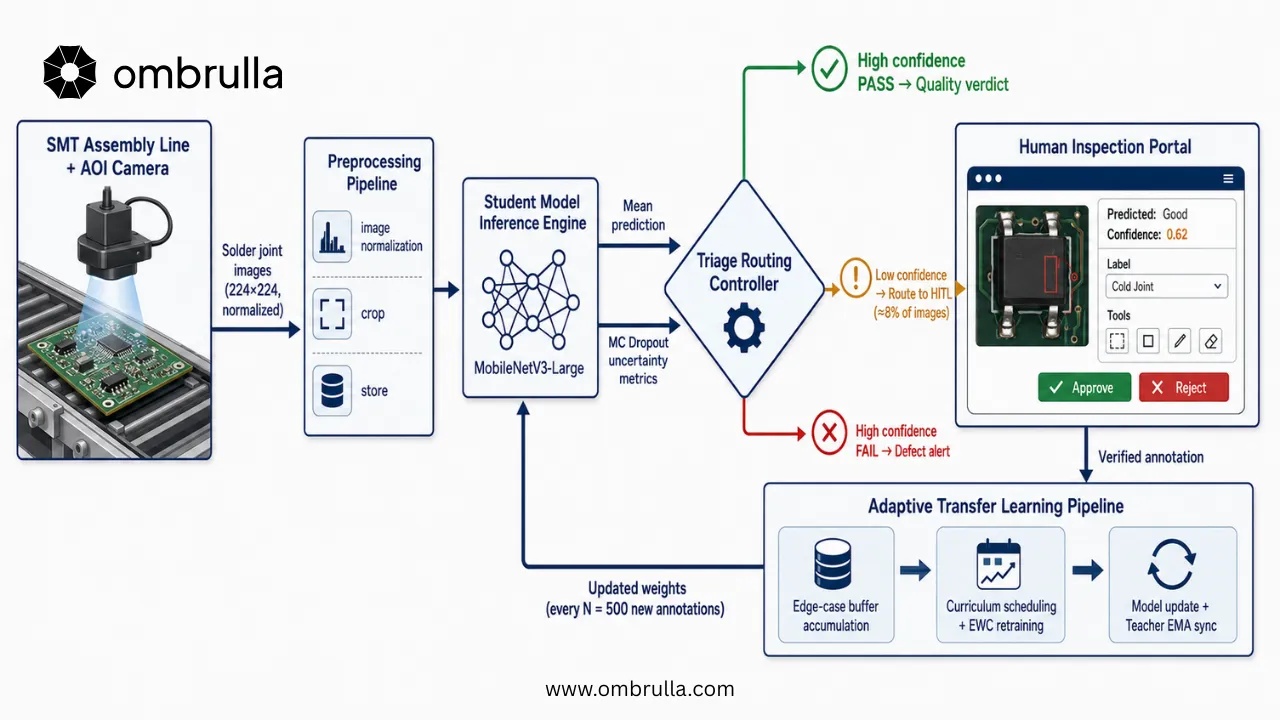
The HITL active learning framework comprises five interacting subsystems that together implement the closed-loop self-correction mechanism at the heart of this AI Quality Control approach. Each subsystem is designed for high throughput, low latency, and seamless integration into existing AOI pipelines. This section provides the architectural overview and data-flow specification.
Five Subsystems
Image Capture and Preprocessing Pipeline: The AOI camera system captures top-down and oblique-angle images of each solder joint at 5-megapixel resolution. Images are normalized, cropped to a 224×224 region of interest centered on the solder joint centroid (determined by the existing AOI system's component placement registry), and stored in a streaming buffer. This preprocessing ensures consistent input dimensions and lighting characteristics for downstream inference.
Student Model Inference Engine: A MobileNetV3-Large backbone, fine-tuned on the initial training dataset, performs batch inference on the image stream. For each image, T = 20 stochastic forward passes with MC Dropout active generate an empirical predictive distribution over the six output classes (acceptable, bridge, open, cold joint, insufficient solder, tombstone), from which the mean prediction and predictive entropy are computed. The lightweight student model architecture ensures high-throughput inference while maintaining competitive accuracy.
Triage Routing Controller: This component compares each image's uncertainty metrics against configurable thresholds and routes images to one of three paths: (1) high-confidence pass-direct quality verdict, no human review; (2) high-confidence fail-immediate defect alert sent to operator; (3) low-confidence route-forwarded to the human AI Inspection portal for expert review. The routing decision is based on composite uncertainty criteria combining predictive entropy and maximum softmax response.
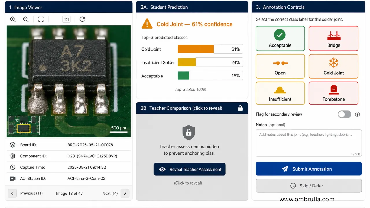
Human Inspection Portal: A web-based operator interface that presents routed images with the student model's prediction, the teacher model's soft-label comparison, and annotation controls. Each review task uses progressive disclosure of information: operators first see only the image and make their judgment, then optionally reveal the model's prediction and teacher comparison. Completed annotations are time-stamped, attributed to the operator, and enqueued for retraining. The portal tracks operator expertise and feedback patterns to optimize task assignment.
Adaptive Transfer Learning Pipeline: A background retraining service that accumulates annotated edge cases, applies curriculum scheduling and elastic weight consolidation (EWC) regularization, updates the student model, and periodically synchronizes the teacher's exponential moving average (EMA) weights. This pipeline implements the key mechanism that closes the loop: human feedback is systematically converted into model improvements without requiring manual intervention or scheduled downtime.
Uncertainty Quantification via Monte Carlo Dropout
Theoretical Foundation
Standard neural network classifiers output a point estimate of class probabilities without any expression of uncertainty about that estimate. A model that assigns 0.73 probability to the 'bridge' class is making a confident prediction, but a practitioner cannot tell from that number alone whether the confidence comes from strong, unambiguous visual evidence or from an uncertain balance among several plausible interpretations.
Monte Carlo Dropout addresses this by treating inference-time dropout as approximate Bayesian inference over network weights, a technique that strengthens the reliability of any downstream Computer Vision decision. The key insight is that dropout applied at test time with stochastic forward passes can approximate the integral over a posterior distribution of network weights.
Formally, let f(x; θ) denote the softmax output of a network with parameters θ and let p(θ | D) be the true posterior over parameters given training data D. A prediction under model uncertainty would ideally compute the integral: ∫ f(x; θ) p(θ | D) dθ, which is intractable for deep networks. MC Dropout approximates this integral by performing T stochastic forward passes with dropout masks active, treating each pass as a sample from an approximate posterior q(θ). The resulting T vectors of class probabilities form an empirical predictive distribution from which uncertainty measures can be computed.
Uncertainty Metrics for Triage Routing
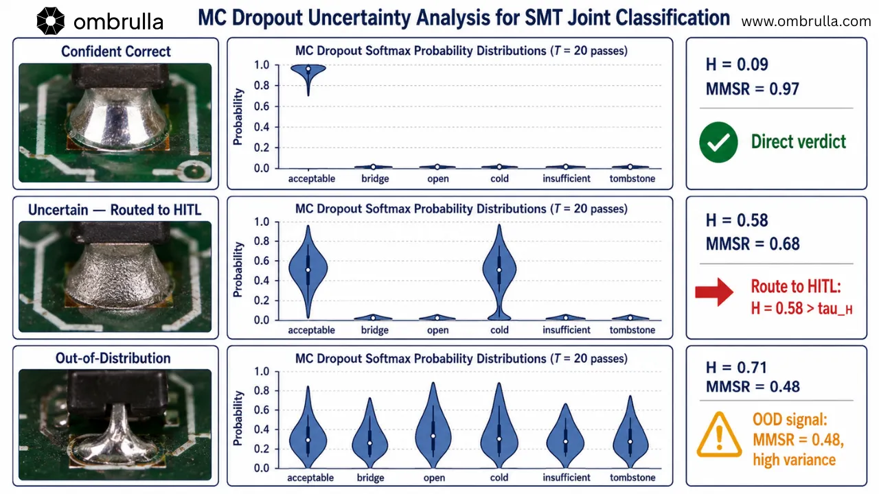
Two complementary uncertainty metrics are computed from the MC Dropout distribution. Predictive entropy H(p̂) measures total uncertainty about the prediction, quantifying how spread the probability mass is across the six defect classes. Maximum Mean Softmax Response (MMSR) measures the peak predicted class probability averaged across the T stochastic passes, indicating the model's confidence in its top-scoring class.
A high predictive entropy combined with a low MMSR indicates genuine model uncertainty about the image's class. A high MMSR with high entropy would indicate inconsistency among MC passes, suggesting an out-of-distribution sample where the model's stochastic samples disagree. The triage routing decision uses a composite criterion: route to HITL if (H(p̂) > τ_H) OR (MMSR < τ_M), where τ_H and τ_M are calibrated per-class thresholds.
In the experimental setup, we use τ_H = 0.40 (in nats) and τ_M = 0.70, calibrated against the validation set to achieve a human annotation budget of approximately 8% of total production images. These thresholds are tuned to prioritize recall over precision, reflecting the 12:1 cost asymmetry of false negatives to false positives identified in Section 3.2.
Computational Cost of MC Dropout
The computational overhead of T = 20 MC Dropout passes relative to a single deterministic pass is roughly 1.8× in practice, thanks to batching efficiency gains that partially offset the linear scaling with T. On the production inference hardware (NVIDIA Jetson AGX Xavier), this yields end-to-end inference throughput of about 340 images per second, which comfortably matches the production line's AOI camera capture rate of 280 images per second.
Twenty-fold uncertainty estimation is therefore achievable without becoming the throughput bottleneck for this AI Inspection pipeline. The latency budget for inference (including preprocessing and triage routing) is approximately 3 milliseconds per image, leaving ample margin for integration with existing AOI systems. This efficiency enables real-time deployment on edge hardware without requiring GPU acceleration for the uncertainty quantification step, though GPU availability further improves throughput.
Student–Teacher Network Design and Knowledge Distillation
Architecture and Rationale
The framework maintains two models in parallel throughout the operational lifecycle. The student model is a MobileNetV3-Large backbone with a custom two-layer classification head, pretrained on ImageNet and fine-tuned on the initial SMT inspection dataset D₀. Its compact architecture (about 5.4 million parameters) enables the fast, batched inference and the T-fold MC Dropout throughput required for production deployment.
The teacher model is a ResNet-50 backbone with an identical classification head (about 25.6 million parameters). The teacher is not deployed in the real-time inference pipeline; it operates in the background during training epochs, supplying soft pseudo-labels for unlabeled production images and supervision for the student's retraining. This size asymmetry is deliberate and serves three functions: (1) the teacher's greater representational capacity enables it to form more nuanced decision boundaries, particularly for visually similar adjacent classes such as cold joints and insufficient solder; (2) it generalizes from fewer examples than the student requires; (3) the student benefits from the teacher's knowledge both indirectly through soft-label signals during distillation training and directly through pseudo-labels on unlabeled images that are not routed to human review.
Mean Teacher Weight Synchronization
Rather than maintaining the teacher as a fixed, separately trained model, the framework uses a Mean Teacher update rule in which the teacher's weights θ_T at training step k are updated as the exponential moving average of the student's recent weight history: θ_T(k) ← α·θ_T(k-1) + (1-α)·θ_S(k), where α = 0.995 is the EMA momentum parameter and θ_S(k) are the student's weights after training step k.
This update rule makes the teacher a temporally smoothed version of the student, which tends to be more stable and better calibrated than the student at any individual training step. By maintaining the teacher as an exponential moving average rather than a separately trained checkpoint, we ensure that the teacher gradually incorporates the student's learning improvements while retaining institutional knowledge about previously mastered defect classes-a key mechanism for mitigating catastrophic forgetting.
The teacher's pseudo-labels on unlabeled images are weighted in proportion to the teacher's own MC Dropout confidence for each image, down-weighting pseudo-labels that the teacher itself is uncertain about. This confidence-weighting scheme prevents the pseudo-labeling process from amplifying errors: images that the teacher struggles with are given less weight during student retraining, focusing gradient updates on examples where the teacher provides reliable supervisory signals.
Knowledge Distillation Loss
The student's training objective combines three loss terms. First, a cross-entropy loss on human-annotated images from the HITL portal: ℒ_CE = -∑_i y_i log(p_student(y_i | x_i)). Second, a knowledge distillation loss measuring the KL divergence between the student's and teacher's softmax outputs, computed at softmax temperature T_kd = 4.0 to soften the teacher's distributions: ℒ_KD = KL(σ_teacher(x; T_kd) || σ_student(x; T_kd)). Third, the elastic weight consolidation regularization term ℒ_EWC described in Section 8.
The combined loss is: ℒ_total = λ₁·ℒ_CE + λ₂·ℒ_KD + λ₃·ℒ_EWC, with weights λ₁ = 1.0, λ₂ = 0.4, and λ₃ = 0.6, tuned on the validation set. The ratio λ₁ > λ₂ ensures that ground-truth human annotations dominate the training signal over pseudo-labels, which is essential for the HITL loop to function as a genuine correction mechanism rather than a self-reinforcing pseudo-labelling cycle. Human feedback is the error signal that drives model improvement; pseudo-labels from the teacher provide regularization and semi-supervised learning benefits, but should not override human judgment.
Dynamic Triage Routing and the Human Inspection Portal
Three-Path Routing Logic
The Triage Routing Controller classifies each inference result into one of three routing paths based on the MC Dropout uncertainty metrics. The High-Confidence Pass path applies when (MMSR ≥ τ_M) AND (H(p̂) ≤ τ_H) AND (predicted class is acceptable): the image receives an automatic pass verdict and no human review occurs. The image proceeds directly to the quality pass log.
The High-Confidence Fail path applies when (MMSR ≥ τ_M) AND (H(p̂) ≤ τ_H) AND (predicted class is a defect): the image receives an automatic fail verdict and is logged with the predicted defect class for operator notification and downstream rework routing. Defect alerts are immediately communicated to production floor supervisors through the AOI system's existing notification infrastructure.
The HITL Route applies when either uncertainty criterion flags the image: (H(p̂) > τ_H) OR (MMSR < τ_M): the image is enqueued for the human inspection portal. These are the edge cases-images where the model's confidence is genuinely low and expert human judgment is most valuable. Typically, 8–10% of production images are routed to HITL under normal operating conditions.
The triage thresholds τ_H and τ_M are not static parameters. Each week, the system evaluates the precision and recall of the previous week's automatic verdicts against a random 2% sample that is sent to human review regardless of confidence (serving as a ground-truth validation set). Based on this evaluation, the thresholds are adjusted to hold a target false negative rate (typically calibrated to no more than 1% escape rate on confidently predicted defects). This dynamic threshold adaptation keeps the triage policy calibrated even as the overall distribution of confidence scores shifts because of model retraining and production drift.
Human Inspection Portal Design
The AI Visual Inspection platform is a browser-based interface built for efficient, low-fatigue annotation of edge-case images by trained quality operators. Each review task presents the operator with four key elements: (1) the solder joint image at full resolution with zoom capability for detailed inspection; (2) the student model's predicted class and confidence percentage; (3) the teacher model's top-two class predictions with confidence comparison; and (4) annotation controls for providing ground truth.
The three annotation options are: confirm the student prediction (single click), select a different class from the taxonomy dropdown (for correcting model errors), or flag as ambiguous for secondary review (for genuinely uncertain cases that may require further investigation or manufacturing record review). Confirmed annotations are time-stamped, attributed to the operator, and immediately enqueued for the retraining pipeline.
A key design principle is progressive disclosure of context. In the default view, the operator sees only the image and the student's prediction, forming their own judgment before the teacher's comparison is revealed with a single click. This prevents anchoring bias in which the operator simply confirms whatever the model predicted, which would defeat the correction function of the HITL loop and undermine the value of this AI Visual Inspection safeguard. By forcing operators to commit to their own visual judgment first, the framework ensures that human annotations represent genuine expert knowledge rather than model compliance.
The portal tracks per-operator precision, recall, and inter-rater agreement statistics, flagging systematic disagreement patterns that may indicate operator fatigue, insufficient training, or ambiguous image quality issues. A progress indicator shows the operator's current position in the queue and session statistics (e.g., '12 of 47 completed this session'). The target annotation rate is 24 images per operator-hour at comfortable working pace, totaling about 20–30 minutes of focused annotation per 8-hour shift when integrated into the operator's routine inspection duties.
Adaptive Transfer Learning and Catastrophic Forgetting Mitigation
Curriculum-Guided Retraining Schedule
New HITL annotations do not immediately trigger a retraining cycle. Instead, annotations are buffered in the edge-case store until either a volume threshold (N = 500 new annotations) or a time threshold (7 days since last retraining) is reached, whichever comes first. This buffering strategy ensures that retraining runs are computationally efficient and that the model benefits from a diverse batch of recent feedback before updating.
At retraining time, the curriculum scheduler assembles a mixed training batch drawn from three sources: (1) new HITL-annotated edge cases (about 30% of each batch)-these are the most recent, highest-value examples; (2) a balanced sample from the original training dataset D₀ (about 40%)-this preserves performance on the original distribution; (3) teacher pseudo-labeled examples from recent unlabeled production images (about 30%)-this provides semi-supervised learning on examples the model is confident about. This mixture prevents the model from over-fitting to the most recent distribution while ensuring new edge cases receive sufficient gradient signal to drive learning.
Within each batch, examples are ordered by curriculum difficulty, starting with high-confidence teacher pseudo-labels and progressing to lower-confidence human-annotated edge cases as the epoch progresses. This easy-to-hard curriculum scheduling, inspired by Bengio et al.'s original curriculum learning proposal, has been shown empirically to improve convergence speed and generalization in continual learning settings. The curriculum strategy ensures that the model first reinforces its understanding of high-confidence patterns before tackling the ambiguous edge cases that define the current drift.
Elastic Weight Consolidation
Elastic Weight Consolidation (EWC) mitigates catastrophic forgetting by adding a regularization term to the training loss that penalizes changes to parameters deemed important for previously learned tasks. The EWC regularizer is: ℒ_EWC = (λ₃/2) ∑_i F̂_i (θ_i - θ*_i)², where θ*_i are the parameter values at the conclusion of the most recent retraining cycle, F̂_i is the diagonal of the empirical Fisher information matrix estimated from a fixed diagnostic set representing all six defect classes, and λ₃ is the EWC regularization strength.
The Fisher information matrix acts as a proxy for parameter importance: parameters with high Fisher information are those most influential for the model's predictions on well-mastered defect classes. By penalizing changes to high-importance parameters, EWC effectively freezes them in place, allowing the model to adapt to new edge cases primarily through parameters that were less important for prior tasks. In the experiments, we use λ₃ = 0.6, which provides a balanced trade-off between learning new defect patterns and preserving existing knowledge.
The Fisher matrix is estimated on a fixed diagnostic set representing all six defect classes in balanced proportions. This ensures that the importance weighting reflects the model's performance across all defect types equally, rather than being biased toward the most common or recently seen classes. Periodic re-estimation of the Fisher matrix (typically every 2–3 retraining cycles) further refines the importance weights as the model's representations evolve.
Retraining Validation Gate
Every candidate updated model must pass a validation gate before it replaces the current production model. The gate evaluates the updated model on a fixed validation set drawn from D₀ (which represents the historical distribution of defect types) and on a recent-production validation set (which represents the current distribution). Both sets must meet minimum recall thresholds for each of the six classes before the updated model is promoted. If the gate fails, the retraining run is logged as unsuccessful, the EWC regularization strength λ₃ is increased by 0.1, and retraining is rescheduled. This gate keeps a degraded model out of production and provides an automatic hyperparameter adaptation mechanism for environments where forgetting is particularly problematic - an important safeguard for any production-grade AI Quality Control system.
Experimental Setup and Dataset
Production Facility and AOI System
The framework was deployed at an electronics manufacturing services (EMS) facility producing industrial control boards with mixed SMT (surface mount technology) and through-hole technology. The AOI (automated optical inspection) system consisted of an inline inspection station processing boards at 280 images per second across three inspection channels: top-down white-light illumination for vertical solder profile assessment, oblique-angle raking light for edge detection and bridging diagnosis, and infrared thermal capture for thermal anomalies and cold joint detection.
The facility operates three production shifts of eight hours each, producing between 4,200 and 6,800 inspectable board assemblies per day, depending on product complexity and order volume. The product mix is diverse, including components from six families: 0402 and 0201 chip passives (resistors, capacitors, inductors), SOT-23 small-signal transistors (BJTs, MOSFETs, diodes), SOP-8 dual in-line ICs (operational amplifiers, voltage regulators), QFP-32 and QFP-48 fine-pitch ICs (microcontrollers, signal processors), and BGA (ball grid array) packages inspected by X-ray augmentation for internal void detection. This heterogeneous product mix is typical of contract manufacturing and represents the real-world challenge of maintaining model performance across diverse component types, package sizes, and board densities.
Dataset Composition
The initial training dataset D₀ was assembled from 18 months of historical AOI images, comprising 142,000 annotated solder joint images. This dataset was curated from multiple sources: acceptable joints from historical AOI pass verdicts, defects from both expert manual labeling by experienced quality engineers and AOI system fail records. The curation process included expert re-verification of ambiguous cases, particularly for cold joints, to ensure high-quality ground truth labels.
| Defect Class | Count | % of D₀ | Annotation Source | Validation Count |
|---|---|---|---|---|
| Acceptable | 93,800 | 66.1% | Historical AOI pass verdicts | 12,400 |
| Solder Bridge | 14,200 | 10.0% | Expert labeling + AOI fail records | 1,880 |
| Open Joint | 9,400 | 6.6% | Expert labeling | 1,250 |
| Cold Joint | 11,100 | 7.8% | Expert labeling (re-verified) | 1,470 |
| Insufficient Solder | 8,600 | 6.1% | Expert labeling | 1,140 |
| Tombstone | 4,900 | 3.4% | Expert labeling | 650 |
| TOTAL | 142,000 | 100% | - | 18,790 |
The class distribution reveals significant imbalance: acceptable joints comprise 66.1% of the dataset, while rare defect classes like tombstoning represent only 3.4%. This imbalance is realistic for production environments (defect rates are typically 1–5%) but motivates the curriculum-weighted batch sampling strategy used in the retraining pipeline: balancing representation across classes during training ensures the model maintains sensitivity to rare but critical defects.
Over the 90-day evaluation period, the production run generated an additional 2.1 million solder joint images. Of these, approximately 8.3% (174,300 images) were routed to the HITL portal during the evaluation period under the configured triage thresholds (τ_H = 0.40, τ_M = 0.70). This HITL routing rate represents a significant operational advantage: without model retraining, an estimated 28.6% of production images would have needed human review under the Month 3 uncertainty distribution-a 3.4× increase in annotation workload that would be operationally infeasible at scale.
Baseline Comparison Systems
We compare the HITL active learning framework against four baselines. The Static Model baseline uses the initial model f_theta trained on D_0 without any retraining throughout the 90-day period. The Periodic Full Retrain baseline simulates the facility's prior practice of complete model retraining at 30-day intervals using all accumulated HITL annotations and a balanced resample of D_0. The Active Learning (No HITL) baseline uses MC Dropout uncertainty sampling to select images for annotation but presents them as a batch at each 30-day interval rather than routing them in real time. The HITL No-EWC baseline uses the full HITL active learning framework but without elastic weight consolidation, to isolate the contribution of forgetting mitigation.
Results and Analysis
Defect Escape Rate
The primary safety-critical metric is the defect escape rate: the fraction of defective joints that receive an automatic pass verdict. Table 2 reports escape rates and F1 scores over 90 days, broken down by system and defect class.
| System | Overall Escape | Cold Joint | Open Joint | F1 Score |
|---|---|---|---|---|
| Static Model (baseline) | 3.84% | 6.21% | 4.17% | 0.881 |
| Periodic Full Retrain (30-day) | 2.95% | 4.83% | 3.02% | 0.909 |
| AL No-HITL (batch, 30-day) | 2.71% | 4.44% | 2.89% | 0.916 |
| HITL No-EWC | 2.31% | 3.81% | 2.14% | 0.923 |
| HITL Active Learning (proposed) | 2.10% | 3.22% | 1.76% | 0.937 |
The 25% reduction in defect escapes (3.84% to 2.10%) represents approximately 0.37 fewer defects per 100 images escaping detection-substantial in terms of field failure prevention. Cold joints show the largest improvement (45% relative reduction), reflecting their sensitivity to reflow and solder paste changes. The EWC contribution is substantial: removing it (HITL No-EWC) increases escape rate by 0.21 percentage points, with particularly large degradation on bridge detection, indicating catastrophic forgetting.
Annotation Efficiency
| System | Total Annotations | Annotation Hours | Annotations per F1 Point |
|---|---|---|---|
| Periodic Full Retrain (30-day) | 84,200 | 421 hours | 8,420 |
| AL No-HITL (batch, 30-day) | 52,400 | 262 hours | 3,920 |
| HITL Active Learning (proposed) | 33,700 | 168 hours | 1,690 |
The 60% reduction in annotation hours (421 to 168 hours) comes from two mechanisms: real-time HITL routing targets effort at uncertain images only, eliminating wasted re-annotation of high-confidence images; and MC Dropout routing selects maximally informative examples consistent with active learning theory. The efficiency metric (annotations per F1 point) shows a 5× improvement: 1,690 vs. 8,420 for periodic retraining.
10.3 Longitudinal F1 Score Trajectory
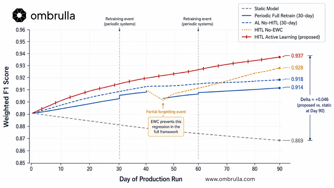
The static model shows steady decline (0.891 → 0.869), demonstrating edge-case drift. Periodic retrain shows staircase pattern with plateaus between updates. AL No-HITL follows similar pattern with slightly smoother transitions. HITL No-EWC rises smoothly to 0.923 but shows visible dip around Day 45-catastrophic forgetting as cold/open joint retraining overwrites bridge parameters. The proposed framework rises smoothly and consistently to 0.937 (Δ = +0.046, or 5.2% improvement), demonstrating sustained learning without forgetting regression.
Discussion: Practical Deployment Considerations, Limitations, and Extensions
Practical Deployment Considerations
Several practical factors shaped the framework design choices that may differ in other deployments. The T = 20 MC Dropout pass count represents a balance between uncertainty estimation quality and inference throughput on the available hardware. Facilities with GPU accelerators offering higher peak throughput could increase T at no latency cost, while constrained edge deployments might use T = 10 with acceptable calibration. The N = 500 annotation buffer threshold was chosen to match the facility's shift pattern, ensuring at least one retraining cycle per production week; a facility with higher throughput and faster drift might target N = 200 for more responsive adaptation.
The 8% HITL routing rate achieved in the evaluation represents about 24 image reviews per operator-hour at the portal, which operators described as a comfortable workload that did not disrupt their primary inspection duties. Facilities with higher defect rates or more severe drift may find routing rates above 15% require dedicated annotation staffing rather than opportunistic use of existing quality engineers.
Limitations
Three limitations of the current framework are worth acknowledging. First, the MC Dropout uncertainty estimator, while well-calibrated on in-distribution data, may not reliably identify all out-of-distribution samples. Specifically, samples that are out-of-distribution in ways that happen to activate high-confidence neurons despite being genuinely novel can pass through triage routing undetected. Spectral normalization or dedicated out-of-distribution detectors could supplement the MC Dropout criterion for facilities with a known risk of genuinely novel defect types.
Second, the EWC Fisher information estimate is computed on a fixed diagnostic set and may not accurately represent parameter importance as the model's representations evolve significantly over multiple retraining cycles. Periodic re-estimation of the Fisher matrix adds computational cost but may improve forgetting mitigation in long-running deployments.
Third, the framework has been evaluated on a single facility with a specific product and process combination; generalizability to substantially different assembly processes, such as chip-on-board or wafer-level packaging, would require validation experiments before broader AI Visual Inspection rollout.
Directions for Extension
The most productive direction for extending this framework is integrating semi-automatic annotation assistance at the inspection portal. Current LLM-based vision models, such as GPT-4V and Gemini Vision, show promising results on PCB defect description tasks and could pre-populate the annotation field with a suggested class and reasoning, which the operator then confirms or overrides. This could further reduce annotation effort while preserving the human verification function that makes the loop genuinely corrective rather than self-confirming - a meaningful step toward more autonomous AI Inspection workflows.
A second extension would apply Bayesian Optimization to the simultaneous tuning of thresholds τ_H, τ_M, and the EWC regularization strength λ₃ across facilities, enabling a cross-facility meta-learning loop.
Conclusion: From Brittle to Self-Correcting AI Inspection
The fundamental challenge in deploying deep learning for SMT solder joint inspection is not building an accurate initial model-that is achievable with modern architectures, Computer Vision techniques, and sufficient training data. The fundamental challenge is keeping the model accurate as the production world slowly changes around it. Edge-case drift is not a failure of the model; it is a failure of the deployment architecture to use the model's own uncertainty as a signal for targeted human feedback.
The self-correcting HITL active learning framework described in this paper addresses this challenge through a principled combination of techniques that are individually well-established but whose integration for continuous production deployment is novel. Monte Carlo Dropout provides an inference-time uncertainty signal at modest computational cost. The student–teacher structure separates production throughput from knowledge quality. Dynamic triage routing directs human attention to exactly the images that matter most for model improvement. Elastic weight consolidation ensures that yesterday's hard-won learning is protected as today's edge cases are incorporated-the combination that makes this AI Visual Inspection framework self-correcting rather than merely automated.
The 90-day evaluation results show that these ideas work in combination at industrial scale: a 25% reduction in defect escapes, a 60% reduction in annotation effort, and a sustained improvement in F1 score that reverses the drift-driven decline observed in the static model baseline. For electronics manufacturers facing the challenge of deploying AI Quality Control across diverse product families and evolving production conditions, the framework offers a path from brittle static models to genuinely adaptive, self-correcting AI Defect Detection intelligence.
References
- Gal, Y., and Ghahramani, Z. 'Dropout as a Bayesian approximation: Representing model uncertainty in deep learning.' ICML, pp. 1050-1059, 2016.[ICML 2016]
- Hinton, G., Vinyals, O., and Dean, J. 'Distilling the knowledge in a neural network.' NeurIPS Deep Learning Workshop, 2014.[NeurIPS 2014]
- Tarvainen, A., and Valpola, H. 'Mean teachers are better role models: Weight-averaged consistency targets improve semi-supervised deep learning results.' NeurIPS, 2017.[NeurIPS 2017]
- Kirkpatrick, J. et al. 'Overcoming catastrophic forgetting in neural networks.' Proceedings of the National Academy of Sciences 114(13): 3521-3526, 2017.[PNAS]
- Settles, B. Active Learning. Synthesis Lectures on Artificial Intelligence and Machine Learning. Morgan & Claypool, 2012.[Morgan & Claypool]
- Gal, Y., Islam, R., and Ghahramani, Z. 'Deep Bayesian active learning with image data.' ICML, 2017.[ICML 2017]
- Sener, O., and Savarese, S. 'Active learning for convolutional neural networks: A core-set approach.' ICLR, 2018.[ICLR 2018]
- Howard, A. et al. 'Searching for MobileNetV3.' ICCV, 2019.[ICCV 2019]
- He, K., Zhang, X., Ren, S., and Sun, J. 'Deep residual learning for image recognition.' CVPR, 2016.[CVPR 2016]
- Usamentiaga, R. et al. 'Automated surface defect detection in metals: A comparative review.' Metals 12(2): 315, 2022.[Metals Journal]
- Farag, W. S. 'Soldering defects detection in surface mount technology circuit boards using deep learning.' Journal of Manufacturing Systems 62: 282-294, 2022.[Journal of Manufacturing Systems]
- Bengio, Y., Louradour, J., Collobert, R., and Weston, J. 'Curriculum learning.' ICML, pp. 41-48, 2009.[ICML 2009]
- Zenke, F., Poole, B., and Ganguli, S. 'Continual learning through synaptic intelligence.' ICML, 2017.[ICML 2017]
- Lakshminarayanan, B., Pritzel, A., and Blundell, C. 'Simple and scalable predictive uncertainty estimation using deep ensembles.' NeurIPS, 2017.[NeurIPS 2017]
- Fang, M. et al. 'RAPS: Robust and accurate PCB solder joint classification based on deep residual networks.' Journal of Intelligent Manufacturing 34: 1841-1855, 2023.[Journal of Intelligent Manufacturing]
- Howard, J. et al. 'Universal language model fine-tuning for text classification.' ACL, 2018.[ACL 2018]
- Settles, B., and Craven, M. 'An analysis of active learning strategies for sequence labeling tasks.' EMNLP, 2008.[EMNLP 2008]
- Li, Z. et al. 'Learning without forgetting.' IEEE Transactions on Pattern Analysis and Machine Intelligence 40(12): 2935-2947, 2018.[IEEE TPAMI]