
The Physics Problem: Motion Blur, Ambient Light Drift, and Specular Reflection
Every AI visual inspection failure that isn't a model problem is usually an imaging problem wearing a model problem's clothes. Three physical effects account for most of it: motion blur, ambient light drift, and specular reflection.
Motion Blur - When Line Speed Outruns Your Exposure Window
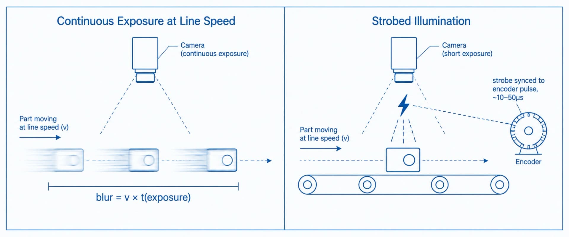
Motion blur is a straightforward geometry problem that often gets treated as a mysterious accuracy problem. A part moving at velocity v across the camera's field of view during an exposure time t travels a distance of v × t during that single frame - and that distance is exactly how blurred the image becomes.
Take a line running at 1.2 m/s, a fairly typical conveyor speed for small assembled parts, with a camera using a continuous exposure of 5 milliseconds. The part moves 6 mm during that exposure - almost certainly larger than the defect you're trying to resolve. To hold blur under 0.1 mm (a reasonable target for a 0.3 mm minimum defect size), exposure time has to drop to roughly 83 microseconds. No continuous-illumination setup captures a usable image at 83 μs without extreme sensor gain, which introduces its own noise problem.
The fix isn't a faster camera - it's decoupling exposure time from illumination duration. A pulsed or strobed light source, triggered by a shaft encoder or photoeye synced to the camera's global shutter, delivers a very short, very bright light burst timed to the exact moment the part is in frame. The camera's nominal exposure setting can stay longer while the actual light-integration window is defined by the strobe pulse width, often 10–50 μs. This is why sub-100ms edge inference conversations always loop back to a strobe controller and an encoder - the model can only be as good as the frame it's given.
Dynamic Ambient Light - The Problem Nobody Puts in the Spec Sheet
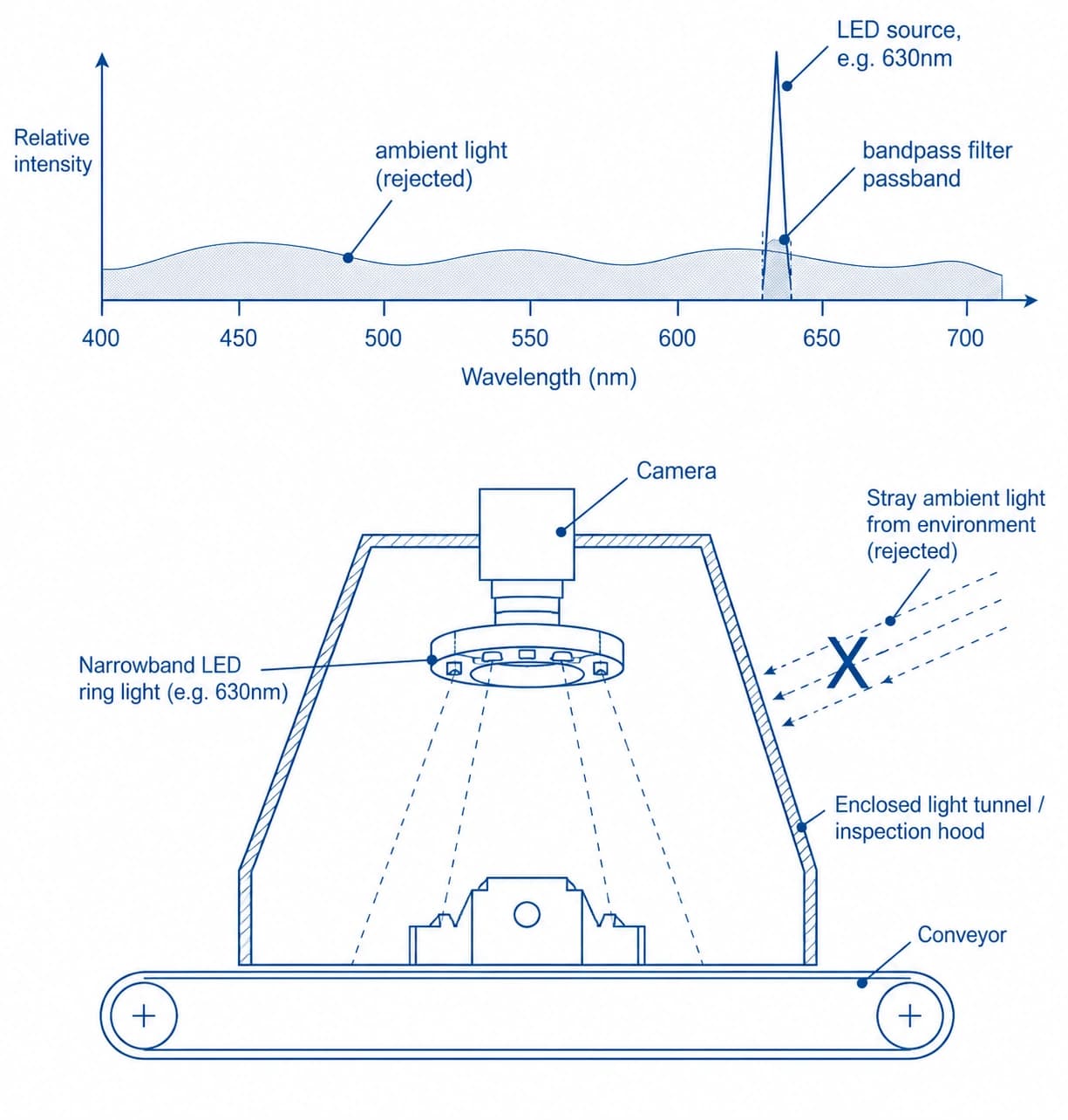
A model validated on a bright Tuesday morning under skylights and idle overhead fluorescents will not perform identically on a Saturday night shift lit only by sodium-vapor high-bays, or next to a bay door left open for forklift traffic. Ambient light contributes both intensity and color-temperature variation that a fixed imaging setup wasn't designed to reject, and it drifts by time of day, weather, and shifts in ways invisible during a short proof-of-concept.
Three responses handle this, in increasing order of robustness and cost: enclosing the inspection zone in a light-tunnel or hood that physically excludes ambient light; using narrowband LED illumination (a specific wavelength, e.g. 630 nm red or 470 nm blue) paired with a matching bandpass filter on the lens, so the camera only accepts light in that band and broadband ambient light is largely rejected; and closed-loop exposure/gain control referencing a fixed calibration target in frame, so the pipeline compensates automatically for slow ambient drift instead of requiring manual recalibration every shift change.
Specular Reflection on Metallic and Glossy Surfaces
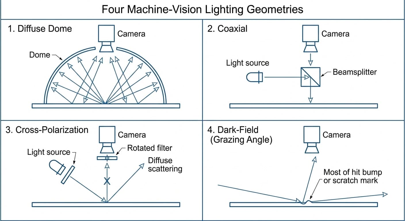
Bare metal, chrome trim, glossy paint, and polished plastic all reflect a point light source directionally rather than scattering it - producing a blown-out hotspot exactly where the camera needs clean signal, and darkness everywhere else. Four lighting geometries solve this depending on what you're trying to see:
- - Diffuse dome (cloudy-day) lightingSurrounds the part with light from every angle, eliminating hard specular hotspots for general surface and cosmetic inspection.
- - Coaxial (on-axis) lightingProjects light through a beamsplitter along the same optical axis as the lens - the standard approach for flat, mirror-like surfaces where dome lighting still leaves off-angle glare.
- - Cross-polarizationPlaces a polarizing filter over the light and a second filter, rotated 90 degrees, over the lens. Specular reflection preserves polarization and gets blocked by the crossed filter; diffuse reflection scrambles polarization and passes through - isolating surface texture and killing glare simultaneously.
- - Dark-field (grazing-angle) lightingDoes the opposite of the above: light aimed nearly parallel to the surface reflects away from the camera on an undamaged, flat area (which appears dark), while a scratch, dent, or pit scatters light directly into the lens and appears bright. This is the standard technique for surface-defect detection on glossy or metallic parts.
Architectural Trade-offs: Edge Accelerators vs On-Prem Clusters for Sub-100ms Inference
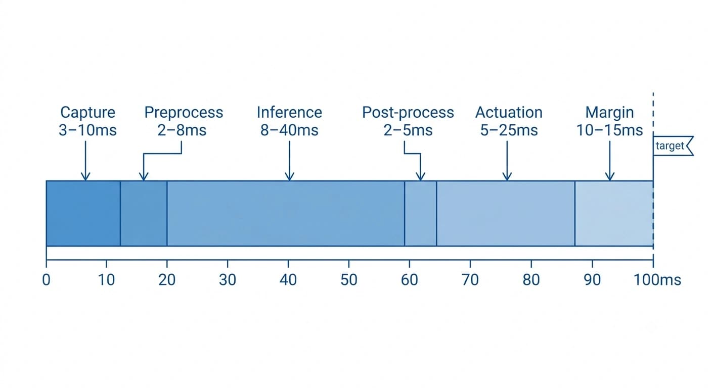
Sub-100ms inference isn't a single number you hit by buying a fast enough GPU - it's a budget you allocate across five sequential stages, and every millisecond spent in one stage is a millisecond unavailable to the others.
Building the Latency Budget
| Stage | Typical Latency | Notes |
|---|---|---|
| Image capture & sensor readout | 3–10 ms | Global shutter reads out faster than rolling shutter; scales with resolution and interface (GigE/USB3/Camera Link). |
| Preprocessing & normalization | 2–8 ms | Cropping, resizing, color correction - CPU or GPU depending on architecture. |
| Model inference | 8–40 ms | Depends heavily on architecture, quantization (FP16/INT8), and accelerator - the stage most vendors optimize, and the one most engineers over-focus on. |
| Post-processing & decision logic | 2–5 ms | Bounding box decoding, confidence thresholding, severity scoring. |
| Actuation signal to PLC/reject mechanism | 5–25 ms | Highly protocol-dependent - hardwired discrete I/O is faster than a networked message. |
| Safety margin | 10–15 ms | Buffered against jitter, GC pauses, thermal throttling. |
Add these up and a well-engineered edge pipeline lands in the 40–90 ms range with margin - but a spec sheet that only reports “model inference: 12 ms” and ignores the other four stages is not describing a deployable sub-100ms system.
Edge Modules vs Centralized GPU Clusters vs Cloud
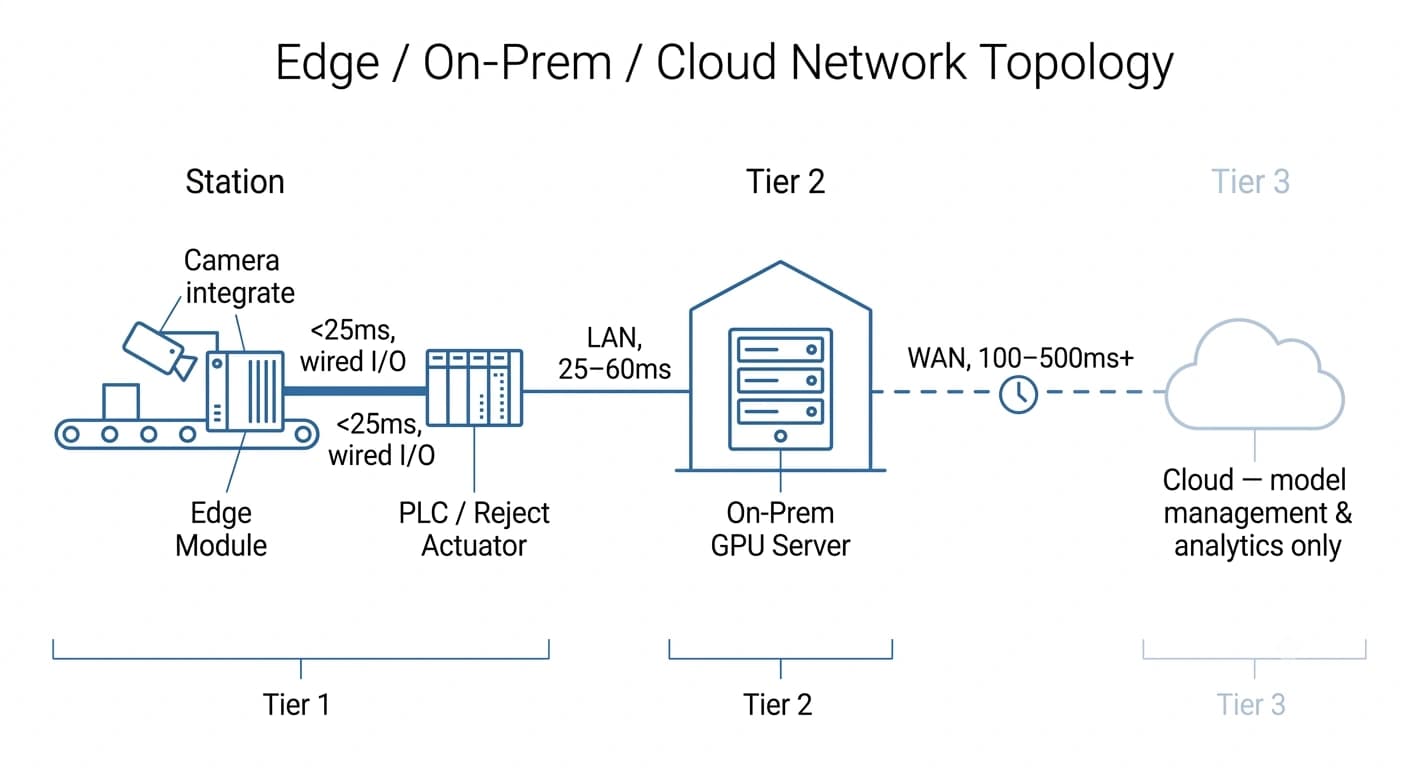
| Dimension | Edge Module (Jetson-class / industrial IPC) | Centralized On-Prem GPU Server | Cloud Inference |
|---|---|---|---|
| Round-trip latency | 15–45 ms | 25–60 ms (LAN-dependent) | 100–500+ ms (WAN-dependent) |
| Per-station hardware cost | Higher - compute duplicated per station | Lower per station - shared, amortized GPU | Lowest capex, ongoing opex |
| Best-fit line speed | High-speed lines needing guaranteed local latency | Multiple medium-speed stations sharing infrastructure | Not viable for the reject decision |
| Offline / air-gapped capability | Full - no network dependency | Requires a reliable LAN to the server room | Not viable |
| Where it fits | The reject/accept decision itself | The reject decision for co-located stations, or training compute | Model management, fleet analytics - never the millisecond-critical path |
The pattern that holds across almost every production deployment: the accept/reject decision lives at the edge, or on a local on-prem GPU server reachable over a low-jitter LAN - never over the internet. Cloud connectivity earns its place for model versioning, fleet-wide analytics, and retraining pipelines, where a few hundred milliseconds of latency is irrelevant. Learn how Ombrulla architects edge-first inference in Tritva.
The Data Pipeline Problem: Class Imbalance, Rare Defects, and Active Learning
Why Defect Detection Breaks Standard Computer Vision Assumptions
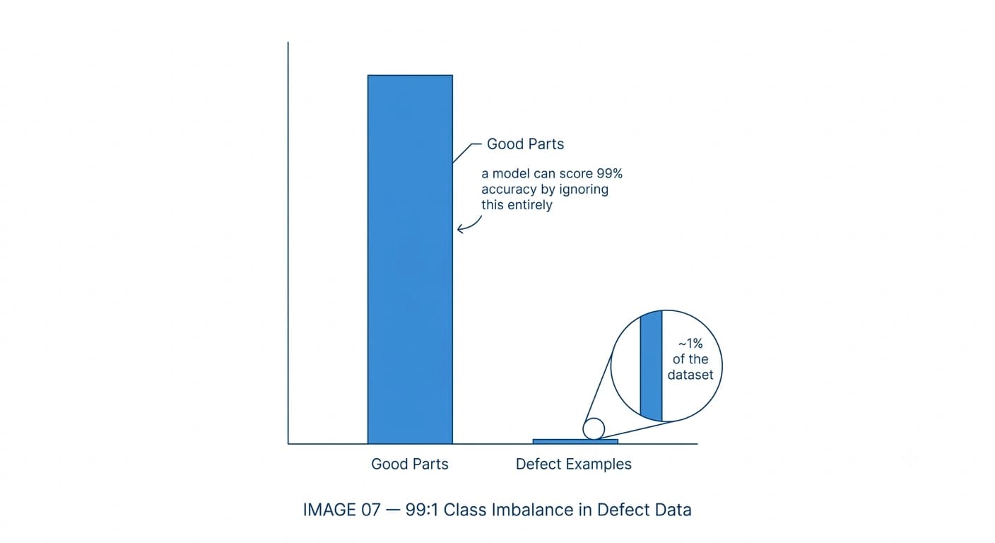
Most computer vision benchmarks assume roughly balanced classes. Manufacturing defect detection almost never is. A well-controlled process might run a 0.1–2% defect rate, which means a dataset built from raw production images is 98:1 to 999:1 imbalanced before a single frame is labeled. A model naively trained on that distribution learns to predict 'good part' for almost everything and still posts a deceptively high accuracy number, because accuracy on an imbalanced dataset is dominated by the majority class.
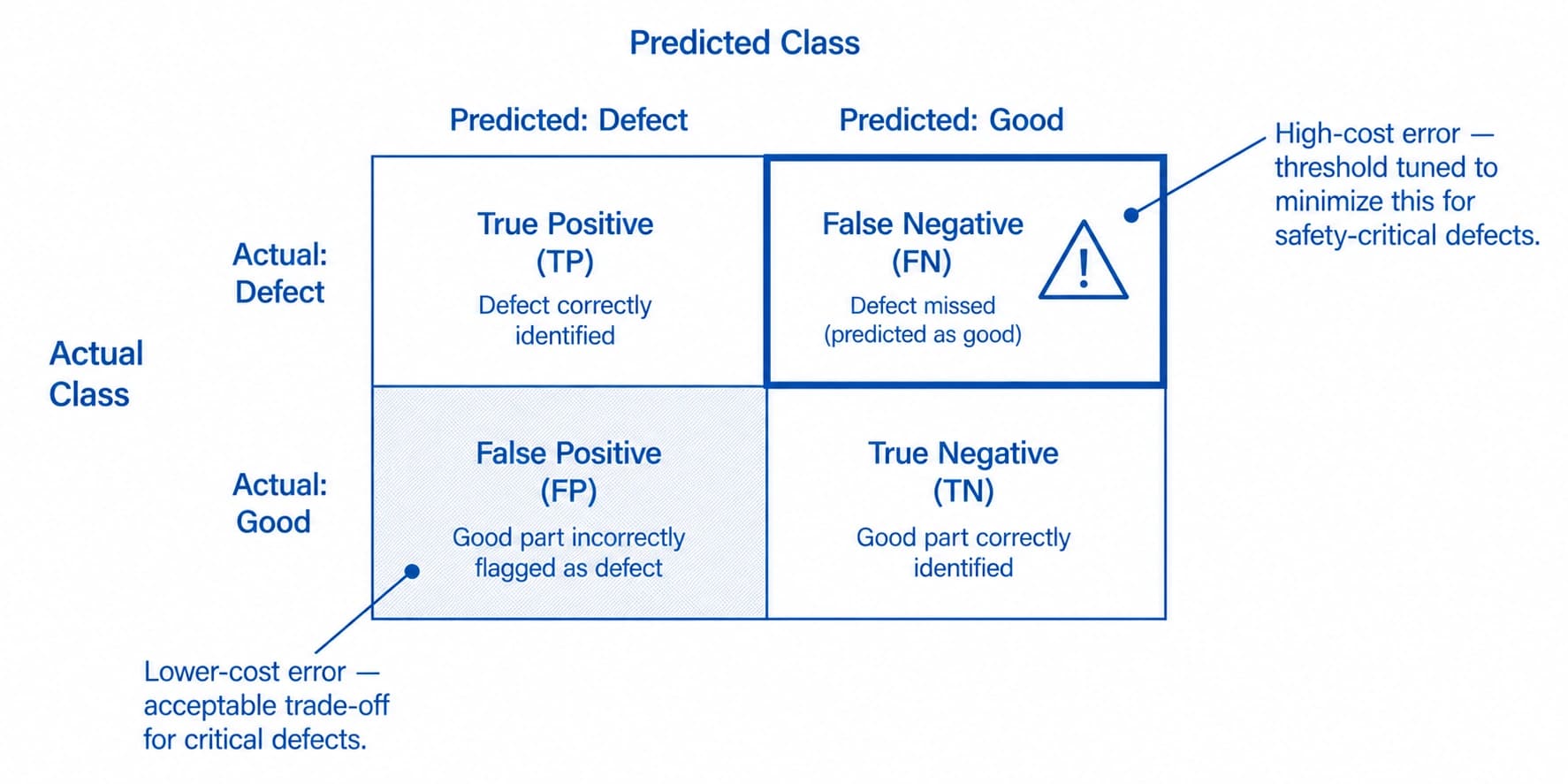
The cost structure compounds the problem: for most safety- or warranty-relevant defects, a false negative (a real defect that ships) costs far more than a false positive (a good part flagged for review) - but standard loss functions treat both errors identically unless told otherwise.
Techniques That Actually Work at 99:1+ Imbalance
- - Class-weighted or focal lossWeighting the loss function inversely to class frequency, or using focal loss to down-weight easy, correctly classified majority-class examples, forces continued learning from rare defect examples instead of early convergence on the easy majority class.
- - Augmentation-based oversamplingRotation, flipping, brightness/contrast jitter, and crop variation applied specifically to minority-class (defect) images multiplies effective coverage without collecting more real defects.
- - Synthetic defect generationGAN- or diffusion-based image synthesis, or simpler procedural compositing of defect textures onto real good-part backgrounds, generates additional minority-class examples for defect types too rare to collect naturally - critical for catastrophic-but-rare failure modes you can't wait months to accumulate.
- - Active learning / uncertainty samplingRather than labeling images at random, the model flags the production images it's least confident about (entropy or margin-based scoring) for labeling priority - concentrating effort on images that move performance the most.
Detecting Data Drift Before It Silently Degrades Your Model
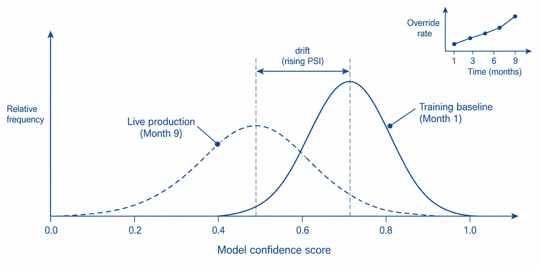
A model doesn't fail loudly when production drifts away from its training distribution - it fails quietly, with confidence scores slowly becoming less trustworthy and an override rate that creeps upward until someone notices. Three techniques catch this early:
- - Population Stability Index (PSI) or KL divergenceCalculated on the distribution of model confidence scores over time - a rising PSI against the training baseline is an early drift signal, often weeks before precision/recall visibly degrades.
- - Periodic re-validation against a held-out labeled reference setRun on a fixed cadence rather than only when someone complains - this catches the gap between 'the model still runs' and 'the model is still accurate.'
- - Embedding-space novelty detectionProjecting incoming images into the model's learned feature space and flagging ones outside the density of the training distribution - catches genuinely new defect types or material changes a confidence check alone would miss, because a model can be confidently wrong about something it's never seen.
Platforms built for this loop turn the retraining cadence into a managed workflow rather than an ad hoc engineering fire drill. Explore continuous retraining tools like Tritva Vision.
Integration Architecture: Speaking the Plant's Native Protocols
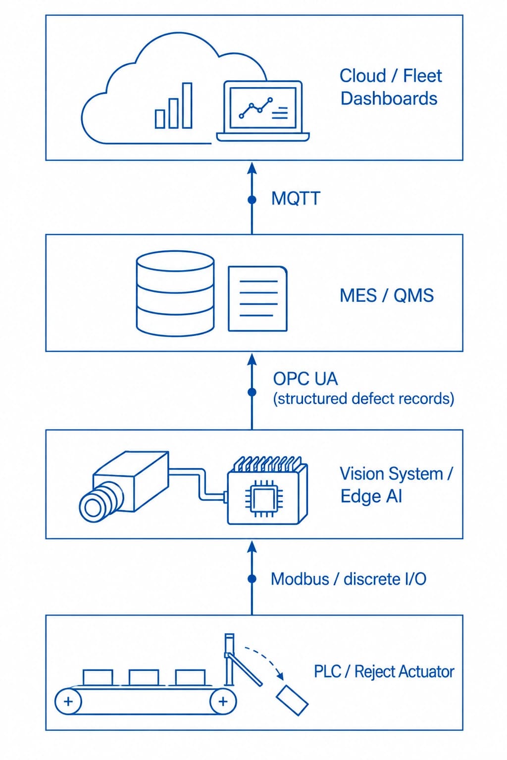
An AI model that can't get its decision into a PLC reject signal or an MES genealogy record in real time isn't a production system - it's an expensive demo. Three protocols cover almost every integration scenario, and they are not interchangeable.
Protocol Comparison for Machine Vision Integration
| Protocol | Data Model | Security | Best Fit | Weakness |
|---|---|---|---|---|
| OPC UA | Rich, self-describing object model; structured data (defect class, severity, image reference, metadata) | Built-in certificate-based auth & encryption | Structured defect records into modern SCADA/MES; multi-vendor interoperability | Higher implementation overhead; needs an OPC UA server/client stack |
| MQTT | Lightweight pub-sub; payload (JSON, Sparkplug B) defined by the app | No native security - relies on TLS/broker-level auth | High-frequency IIoT telemetry, cloud/edge messaging, fleet dashboards | Weaker built-in data modeling; security must be layered on deliberately |
| Modbus | Simple register-based master/slave; raw registers/coils only | None native - isolated physically or by network in practice | Discrete I/O: trigger signals, reject actuation, legacy PLC compatibility | Cannot carry rich defect metadata; request-response only |
In practice, most integrations use more than one: Modbus or a hardwired discrete signal for the millisecond-critical reject actuation, OPC UA for writing the structured defect record into the MES/QMS, and MQTT for streaming aggregate line-health telemetry to a fleet dashboard. Picking one protocol for every layer usually means using the wrong tool for at least one of the three jobs.
Trigger Synchronization - Hardware vs Software
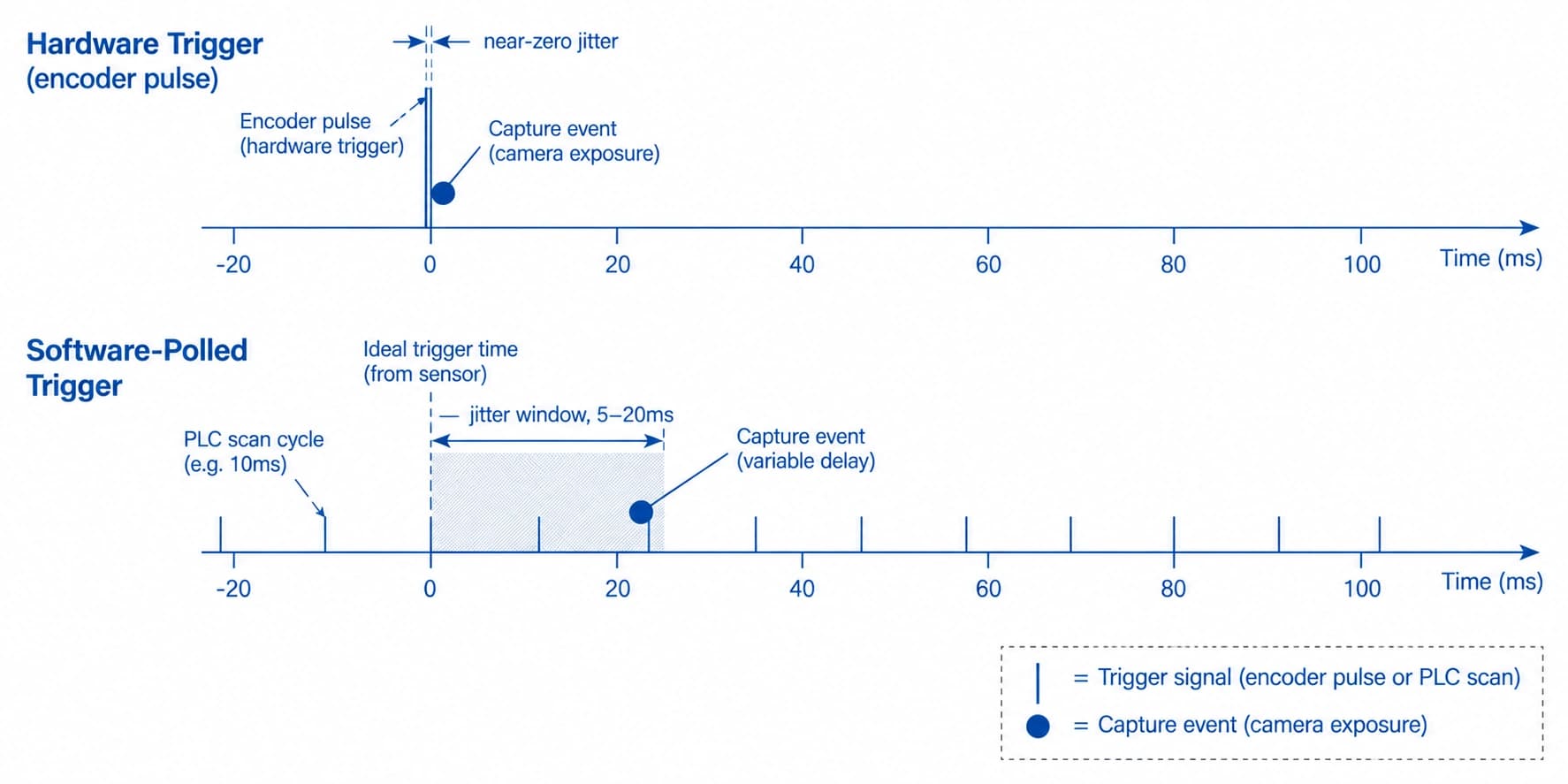
The camera needs to know exactly when a part is in frame, and this is a timing problem, not a software problem. A hardware trigger - a shaft encoder pulse or photoeye break wired directly into the camera or strobe controller - fires with microsecond-level determinism regardless of what else the system is doing. A software-polled trigger, where a PLC or industrial PC checks a sensor state on a scan cycle and issues a capture command, introduces jitter on the order of one to several PLC scan cycles (often 5–20 ms) - usually fine at low line speeds, and usually the hidden cause of intermittent 'missed part' complaints at higher ones. Rule of thumb: if line speed and part spacing leave less than roughly 50 ms of positional tolerance, use a hardware trigger.
Writing Results Back Into the MES/QMS Without Manual Re-Entry
A defect record only has traceability value if it's linked to the specific unit it describes - mapped to a serial number, work order, or lot code the moment it's generated, not in a nightly batch reconciliation. In practice this means an OPC UA method call or a REST webhook fired at inspection time, carrying the unit identifier, defect classification, severity score, confidence, and an image reference, written directly into the MES's genealogy table. Review documented integration patterns for common PLC and MES platforms.
Model Validation Beyond Accuracy: Precision/Recall Under Production Drift
Why Aggregate Accuracy Lies to You
A single 'model accuracy: 98.7%' figure is close to meaningless for a defect-detection model, for the same reason it's meaningless for any severely imbalanced classification problem: if 99% of parts are genuinely good, a model that never flags anything would score 99% and catch zero defects. The metrics that matter are computed per defect class, not in aggregate: precision and recall for each defect type, with the threshold for each one set to the actual cost asymmetry of that defect - a safety-relevant structural crack warrants a threshold tuned to minimize false negatives even at the cost of more false positives; a minor cosmetic blemish on a non-visible surface warrants the opposite.
Designing a Statistically Valid Shadow-Mode Test
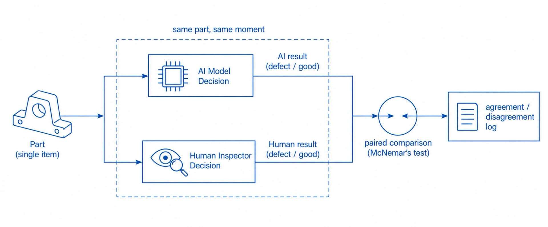
'Run it in shadow mode for a few weeks' is a start, not a validation methodology. Two adjustments make it rigorous. First, calculate the sample size needed to detect a meaningful difference in defect-catch rate with acceptable statistical power before starting, rather than picking a calendar duration arbitrarily - a rare defect class occurring at 0.3% frequency needs a proportionally larger sample of parts to generate enough instances to compare against. Second, when comparing the AI's decisions against a human inspector's decisions on the same parts, McNemar's test - not a simple side-by-side percentage comparison - is the correct statistical tool, because the two decision-makers are evaluating the same paired observations rather than independent samples; an unpaired test here systematically understates or overstates the significance of the difference.
Explore Tritva's shadow-mode validation dashboards for paired statistical testing in live environments.
Emerging Technical Frontiers for 2026
Vision Transformers vs CNNs - Production Readiness Check
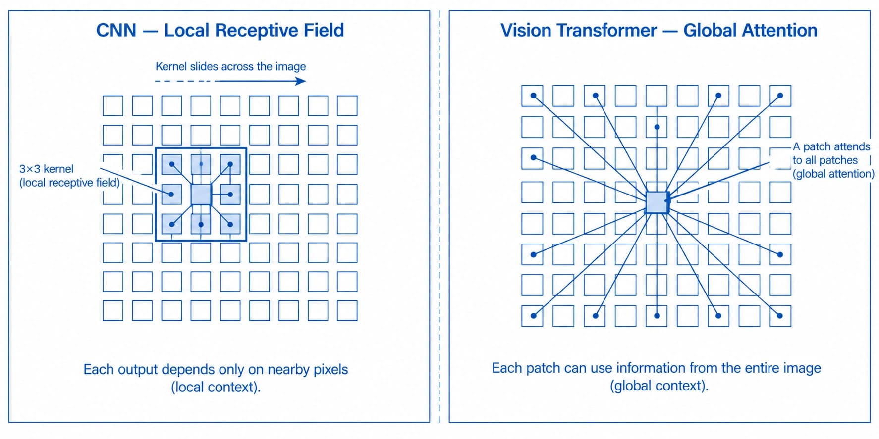
Vision transformers (ViTs) capture long-range spatial dependencies that convolutional architectures structurally can't - useful for pattern-based defects like weave irregularities in textiles or repeating structural anomalies across a large surface. In practice, most 2026 production deployments still lean on CNN backbones (EfficientNet-, YOLO-, and MobileNet-family architectures) for the edge inference stage, because ViTs typically demand more training data and more compute per inference to match CNN accuracy - a real constraint against a sub-100ms, edge-hardware latency budget. Hybrid architectures pairing a lightweight CNN backbone with transformer-based attention for specific defect classes are the more common 2026 production pattern than pure ViT deployment at the edge.
Self-Supervised Pretraining for Rare Defect Classes
Self-supervised methods - masked-image-modeling approaches like MAE, and contrastive approaches like DINO - let a model learn general visual representations from large volumes of unlabeled production images (the images already generated by every good part that's gone down the line) before fine-tuning on the comparatively small set of labeled defect examples. This materially reduces the labeled-example requirement for a usable model on rare defect classes, exactly the constraint that makes catastrophic-but-rare failure modes hard to train for using labeled data alone.
Multimodal Fusion - Vision Plus Acoustic and Thermal
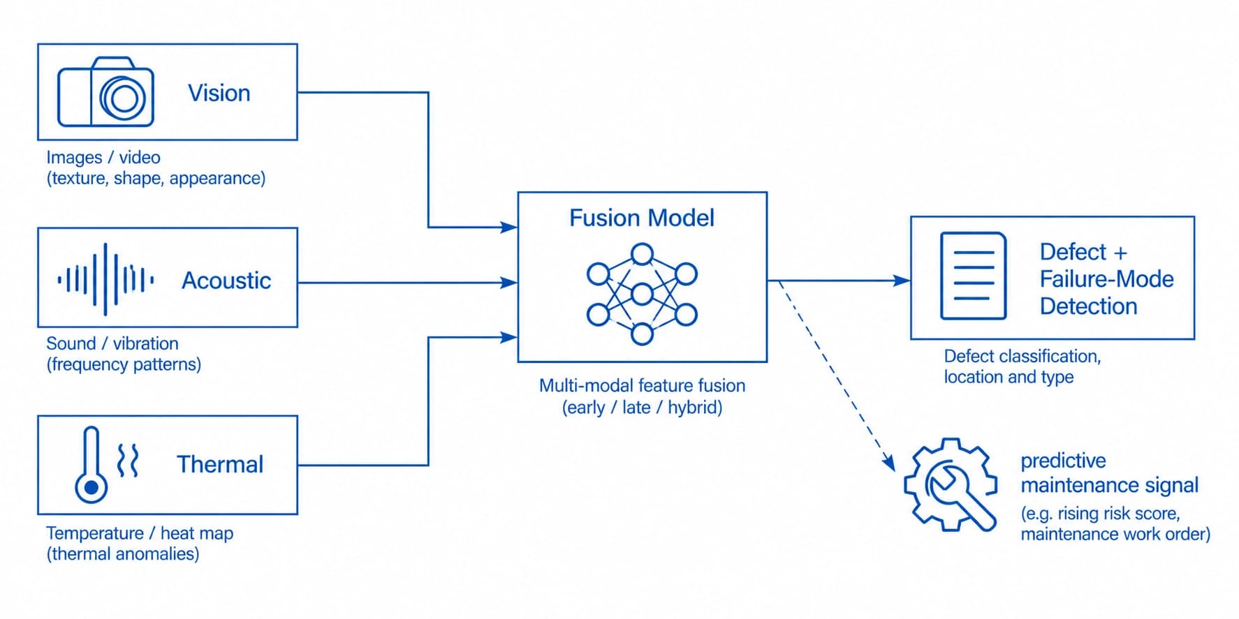
Some failure modes simply aren't visible. A bearing beginning to fail produces an acoustic signature and a thermal signature well before any visible deformation reaches the part surface. Fusing vision inspection data with acoustic and thermal sensor streams - and, further upstream, with the equipment condition data a predictive maintenance system already collects - closes a loop vision alone cannot: correlating a rising defect rate on a specific part feature with the specific piece of equipment and failure mode producing it. This is the direction most enterprise industrial AI stacks are heading in 2026: not a smarter camera in isolation, but a shared data layer across quality and reliability systems.