Industrial AI Predictive Maintenance Benchmark Report 2026 | Pumps, Compressors, CNC & Transformers

Executive Summary

Industrial AI-powered predictive maintenance (AI PdM) has moved well beyond proof-of-concept. In 2026, it is a production discipline deployed across thousands of manufacturing sites, utilities and process plants worldwide. Yet despite market maturity, many organisations still lack a reliable reference point: What ROI should we realistically expect? Which failure modes does AI actually detect - and which does it miss? How do lead times and false alarm rates compare across asset classes?

This benchmark report answers those questions with data drawn from industry studies, OEM technical documentation, peer-reviewed research and verified real-world deployments covering four critical asset classes: centrifugal pumps, rotary compressors, CNC machining centres and power transformers. Our goal is to give plant engineers, reliability managers, OT/IT leaders and digital transformation executives the evidence-based reference they need to make confident investment decisions.

KEY BENCHMARK FINDINGS AT A GLANCE:

-
20–40% Maintenance Cost ReductionPredictive maintenance helps reduce maintenance spend by moving from reactive repairs to planned, condition-based interventions.
-
3–21 Days Early Failure WarningIndustrial PdM systems can provide actionable alerts days or weeks before failure, depending on asset type, sensor coverage, and failure mode.
-
3–10% Optimised False Alarm RateWith proper tuning, rule refinement, and operational feedback, false alarms can be reduced to a manageable industrial range.
-
12–24 Months ROI PaybackWell-scoped PdM deployments typically achieve payback within one to two years through lower downtime, fewer emergency repairs, and improved maintenance planning.

Why 2026 Is a Pivotal Year for Industrial AI PdM

The convergence of edge AI hardware, affordable MEMS sensors, open IIoT connectivity standards and mature machine learning frameworks has produced a step-change in what is achievable on the plant floor. In 2022, most deployments were still confined to pilot programmes on a handful of critical assets. In 2024, large manufacturers began rolling out AI PdM at scale. By mid-2026, according to multiple industry trackers, the global AI-in-predictive-maintenance market surpasses USD 9 billion - with compound annual growth rates exceeding 30%.

But scale has also brought hard lessons. Poorly configured systems generate alert fatigue. RUL predictions made without sufficient training data mislead maintenance planners. ROI projections built on vendor case studies rather than operational benchmarks disappoint CFOs. This report exists to cut through the noise.

Global AI Predictive Maintenance Market 2021–2026: Bar chart showing growth from $2.1B to $9.3B with CAGR trajectory

Scope and Methodology

This report synthesises findings from:

-
Peer-reviewed studies published in IEEE Transactions on Industrial Electronics, Mechanical Systems and Signal Processing, and Reliability Engineering & System Safety
-
OEM technical documentation from major pump, compressor, CNC and transformer manufacturers
-
Field data from industrial IoT platform providers covering deployments across oil and gas, power generation, automotive manufacturing and water utilities
-
Expert interviews with reliability engineers and AI solution architects in Europe, North America and the Middle East

All ROI and cost reduction figures are expressed as ranges rather than single-point estimates to reflect operational variability. Vendor-provided case studies were cross-referenced against independent sources before inclusion.

Centrifugal Pumps

Why Pumps Are the Most Common AI PdM Use Case

Centrifugal pumps are arguably the most ubiquitous rotating machine in industry. From water treatment to petrochemical processing, they operate continuously, often in harsh environments, and account for approximately 25–50% of electricity consumption in process industries. Their failure has cascading consequences: production downtime, environmental incidents and safety hazards. This makes them both a high-value AI PdM target and a well-researched benchmark asset.

Common Failure Modes - Pumps

Failure Mode	Frequency	Primary Sensor Signal	Typical Lead Time
Bearing degradation	~42% of failures	Vibration (HFE)	7–21 days
Seal leakage/failure	~22%	Vibration + pressure	3–10 days
Impeller wear/cavitation	~18%	Vibration + flow delta	5–14 days
Misalignment	~10%	Vibration (1X, 2X)	14–30 days
Motor winding insulation	~8%	Current + temperature	10–28 days

Key Sensor Parameters - Pumps

-
Vibration (triaxial accelerometer, 0–10 kHz): Primary diagnostic tool. High-frequency envelope analysis (HFE/BPFO/BPFI) detects bearing damage weeks before failure.
-
Temperature (bearing housing, motor winding, fluid outlet): Useful secondary indicator. Rapid rise above baseline often confirms active degradation.
-
Motor current signature analysis (MCSA): Detects rotor bar cracks, winding faults and mechanical load anomalies with no additional physical sensor hardware.
-
Differential pressure (inlet vs. outlet): Hydraulic performance indicator. Deviation from pump curve indicates internal wear or cavitation onset.
-
Flow rate correlation: Combined with pressure, enables efficiency trending - key early indicator of impeller degradation.

ROI Benchmarks - Pumps

-
Average unplanned downtime avoided: 68 hours/pump/year in process industries
-
Maintenance cost reduction: 28–38% compared with time-based schedules
-
Bearing replacement cost avoidance: USD 8,000–45,000 depending on pump size
-
Catastrophic failure avoidance: USD 250,000–2M per event (seal failure leading to leak/fire)

Rotary Compressors

The Criticality of Compressor Health

Industrial compressors - screw, reciprocating, centrifugal and scroll types - are the backbone of compressed air systems, refrigeration, gas transmission and process gas applications. A compressor failure in an automotive assembly plant can halt production lines that cost USD 10,000–50,000 per idle hour. In natural gas processing, an unexpected trip can create regulatory, safety and environmental consequences far exceeding the replacement cost of the machine.

Common Failure Modes - Compressors

Failure Mode	Frequency	Primary Sensor Signal	Lead Time
Screw rotor bearing wear	~35%	Vibration (mesh freq.)	10–25 days
Valve failure (reciprocating)	~28%	Vibration + pressure pulse	3–8 days
Oil degradation/contamination	~15%	Oil quality sensor + temp	14–45 days
Intercooler fouling	~12%	Differential pressure + temp	20–60 days
Surge/stall (centrifugal)	~10%	Flow + pressure + vibration	Seconds–minutes

Key Sensor Parameters - Compressors

-
Vibration: Critical for rotating element diagnostics. Screw compressor AI models use rotor mesh frequency, gear mesh frequency and bearing characteristic frequencies.
-
Discharge temperature and pressure: Elevated discharge temperatures indicate valve leakage or fouled intercoolers. Pressure differential trending is highly effective.
-
Oil quality sensors (viscosity, water content, particle count): The most underutilised and highest-value sensor stream. AI models correlating oil trends with vibration predict bearing failures 30–45 days ahead.
-
Current and power consumption: Efficiency degradation analysis. A 3–5% increase in specific power often precedes valve failure by 7–14 days.
-
Suction and interstage pressures (reciprocating): Valve leakage diagnosis. AI algorithms trained on P-V diagram deviations detect individual valve degradation with high precision.

ROI Benchmarks - Compressors

-
Maintenance cost reduction: 30–42% vs. time-based maintenance
-
Avoided unplanned downtime: 45–80 hours/compressor/year in manufacturing
-
Energy savings from efficiency monitoring: 5–12% reduction in compressor energy consumption
-
Valve replacement lead time extension: Average 3.2x increase in useful valve life with AI-guided replacement

CNC Machining Centres

Precision Manufacturing and the Cost of Unscheduled Stops

CNC machining centres - milling, turning, drilling and grinding machines - are the precision workhorses of automotive, aerospace and electronics manufacturing. Unlike pumps and compressors where failure typically means lost production time, CNC failures can also mean scrap production, tooling damage, workpiece rejection and jig or fixture damage. The cost picture is therefore more complex and, in many cases, significantly higher per event.

AI predictive maintenance for CNC is also technically distinct: the machine itself changes state constantly (different operations, tool paths, materials) making signal normalisation more complex and requiring more sophisticated contextual AI models.

Common Failure Modes - CNC Machines

Failure Mode	Frequency	Primary Sensor Signal	Lead Time
Spindle bearing degradation	~38%	Vibration + temperature	5–18 days
Tool wear/breakage	~30%	Current + acoustic emission	Minutes–hours
Feed drive ball screw wear	~15%	Current + positional error	20–60 days
Linear guide degradation	~9%	Vibration (low freq.)	30–90 days
Coolant system failure	~8%	Temperature + flow	2–7 days

CNC machining centre with holographic AI overlay showing vibration spectrum, temperature heatmap, tool wear progression and RUL gauge at 72%

Key Sensor Parameters - CNC Machines

-
Vibration (spindle-mounted accelerometer, high-frequency): Gold standard for spindle bearing health. Defect frequencies at BPFI, BPFO and rolling element pass within 1–20 kHz are primary AI targets.
-
Motor current (spindle and feed drives): Tool wear monitoring. Gradual current increase indicates increasing cutting forces from tool degradation. Sudden spikes indicate tool breakage.
-
Acoustic emission (AE sensors, 100 kHz–1 MHz): Highly sensitive early detection of tool chip formation, micro-cracks and surface deformation. Cost-effective with modern MEMS AE sensors.
-
Positional feedback (servo encoder data): Ball screw and linear guide wear produces measurable positional error trends that AI models can detect through CNC controller data.
-
Thermal mapping (infrared or thermistor arrays): Spindle thermal drift compensation and coolant flow monitoring.

ROI Benchmarks - CNC Machines

-
Scrap reduction: 15–35% reduction in machining rejects from improved tool life management
-
Spindle repair/replacement avoidance: USD 25,000–120,000 per spindle rebuild avoided
-
Maintenance cost reduction: 22–38% compared with scheduled maintenance
-
Overall Equipment Effectiveness (OEE) improvement: 8–18 percentage points from unplanned downtime reduction

Power Transformers

The Most Expensive Asset to Fail

Power transformers - particularly transmission-class units rated at 100 MVA and above - represent some of the highest-value assets in industrial and utility infrastructure. A single unit can cost USD 2–10 million, have a 40–60 week lead time for replacement and, when it fails catastrophically, can trigger grid instability, fire, environmental contamination and regulatory action. The case for AI predictive maintenance is therefore both economically and operationally compelling.

Transformer AI PdM is distinct from rotating machinery monitoring. The primary diagnostic technique is Dissolved Gas Analysis (DGA), complemented by insulation diagnostics, thermal monitoring and oil quality parameters. AI models for transformers typically employ a combination of time-series anomaly detection and physics-informed machine learning.

Common Failure Modes - Transformers

Failure Mode	Frequency	Primary Sensor Signal	Lead Time
Insulation degradation (thermal)	~32%	DGA (CO, CO2) + thermal	30–180 days
Partial discharge (PD)	~22%	DGA (H2) + acoustic + UHF	60–365 days
Tap changer mechanical fault	~20%	DGA + vibration + current	7–45 days
Oil degradation/moisture ingress	~15%	Oil quality (dissolved moisture)	30–90 days
Winding deformation (through-fault)	~11%	Frequency response analysis	After event (immediate)

Key Sensor Parameters - Transformers: DGA Focus

Dissolved Gas Analysis is the cornerstone of transformer condition monitoring. Modern online DGA monitors provide continuous streaming data that AI models can interpret far more powerfully than periodic laboratory tests.

Gas	Fault Indicated	Threshold Alert (IEC 60599)	AI Enhancement
H2	Partial discharge, corona	>100 ppm (mineral oil)	Rate-of-change trending
CH4	Low-temperature thermal fault	>120 ppm	Multi-gas correlation
C2H2	Arcing (high-energy)	>3 ppm	Duval Triangle AI classification
C2H4	High-temperature thermal fault	>90 ppm	RUL regression model
CO	Paper insulation degradation	>870 ppm	CO/CO2 ratio tracking
CO2	Paper insulation overheating	>10,000 ppm	Thermal model correlation

Additional Transformer Sensor Streams

-
Winding hot-spot temperature (fiber optic sensors or thermal model): Primary driver of insulation ageing rate. AI models apply the Arrhenius equation to continuously recalculate insulation life consumption.
-
Dissolved moisture in oil (online sensors): Moisture accelerates insulation degradation. Relative saturation is more meaningful than absolute moisture content due to temperature dependence.
-
Load and ambient temperature data: Essential context for AI models to distinguish thermally-driven gas generation from genuine fault signatures.
-
Vibration (on-load tap changer): Identifies contact wear, drive mechanism looseness and spring fatigue in OLTC mechanisms.

ROI Benchmarks - Transformers

-
Catastrophic failure avoidance: USD 2–50M per event (asset replacement + consequential losses)
-
Maintenance cost reduction: 35–45% vs. periodic inspection schedules
-
Extended transformer life through optimised loading: 5–15 years additional service life with AI-guided thermal management
-
Avoided emergency replacement lead time: 40–60 weeks removed from critical risk

Cross-Asset Sensor Parameter Benchmarks

Understanding which sensor streams provide the highest diagnostic value across asset classes enables organisations to prioritise instrumentation investment. The following matrix summarises our benchmark findings on sensor effectiveness, cost and deployment complexity.

Sensor Type	Pumps	Compressors	CNC	Transformers	Avg. Cost
Vibration	★★★★★	★★★★★	★★★★★	★★☆☆☆	$200–800
Temperature	★★★☆☆	★★★★☆	★★★☆☆	★★★★★	$50–300
Current (MCSA)	★★★★☆	★★★★☆	★★★★★	★★☆☆☆	$100–400
Pressure	★★★★☆	★★★★★	★★☆☆☆	★★☆☆☆	$150–600
Oil Quality	★★★☆☆	★★★★★	★☆☆☆☆	★★★★★	$500–3000
DGA (online)	N/A	N/A	N/A	★★★★★	$5k–25k
Acoustic Emission	★★★☆☆	★★☆☆☆	★★★★☆	★★★☆☆	$300–2000

Alert Lead Time Analysis

Alert lead time - the window between an AI system's first alert and the point of functional failure - is perhaps the single most operationally significant metric in predictive maintenance. It determines whether there is sufficient time for parts procurement, scheduling and safe intervention.

Grouped bar chart comparing AI predictive maintenance alert lead times for pumps, compressors, CNC machines, and transformers across early, typical, and late detection ranges, with transformers showing the longest lead times.

Asset	Failure Mode	Lead Time Range	Operational Significance
Pump	Bearing fault	7–21 days	Typically sufficient for planned shutdown
Pump	Seal failure	3–10 days	Tight window - parts pre-staging critical
Compressor	Valve wear	3–8 days	Requires stocked spare valves on-site
Compressor	Oil degradation	14–45 days	Comfortable planning window
CNC	Spindle bearing	5–18 days	Spindle rebuild must be scheduled
CNC	Tool wear	Minutes–hours	Real-time intervention only
Transformer	Partial discharge	60–365 days	Enables planned replacement programme
Transformer	Tap changer wear	7–45 days	OLTC inspection can be planned

Benchmark Insight: Untapped Lead-Time Potential

The gap between the first detectable degradation signal and the point of no return is often 3–5x longer than the gap between a typical AI alert and actual failure. This means that many current PdM systems are still detecting failures later than technically possible. With improved signal processing, feature engineering, sensor fusion, and model tuning, AI systems can extend actionable maintenance lead times well beyond today’s benchmark averages.

ROI Model and Financial Framework

The Total Value Architecture of AI PdM

A robust ROI model for industrial AI PdM must capture value across four dimensions: direct cost savings, indirect operational benefits, risk mitigation and strategic advantages. Many organisations underinvest in AI PdM because their business cases only model direct maintenance cost savings, missing 60–70% of the total value.

Value Category	Components	Typical % of Total Value
Direct Maintenance Savings	Labour, parts, consumables reduction	25–35%
Downtime Avoidance	Lost production, restart costs, penalties	35–45%
Asset Life Extension	Deferred capital replacement	10–20%
Risk & Compliance	HSE incidents, environmental fines, insurance	10–15%
Energy Efficiency	Optimised loading, reduced losses	5–10%

Simplified ROI Calculation Framework

The following formulas provide a reproducible starting point for building a site-specific AI PdM business case:

-
Annual Value = (N_assets × Avg_downtime_avoided_hrs × Production_rate_$/hr) + (N_assets × Avg_maintenance_saving_$/asset) + (Catastrophic_failure_probability × Consequence_cost_$) + (Energy_saving_% × Annual_energy_spend_$)
-
Net ROI (%) = (Annual Value − Annual Platform Cost) ÷ Total Implementation Cost × 100
-
Payback Period (Months) = Total Implementation Cost ÷ (Monthly Value − Monthly Platform Cost)

Flow diagram presenting a simplified ROI framework for AI predictive maintenance, showing annual value calculation, ROI percentage formula, and payback period estimation based on downtime reduction, maintenance savings, failure avoidance, and energy savings.

Benchmark ROI Data by Asset Class

Asset Class	Impl. Cost Range	Annual Value Range	Typical Payback	5-Year ROI
Pump (per unit)	$3k–15k	$18k–85k	3–10 months	400–900%
Compressor (per unit)	$8k–35k	$45k–250k	4–12 months	350–800%
CNC Machine (per unit)	$5k–25k	$25k–130k	6–18 months	250–650%
Transformer (per unit)	$15k–80k	$100k–2M+	6–24 months	500–2000%+

Maintenance Cost Reduction Ranges

Maintenance cost reduction is the most frequently cited KPI in AI PdM business cases, yet it is also the most widely misrepresented. Headline figures of '50–70% cost reduction' typically reflect cherry-picked single-asset case studies rather than site-wide averages. Our benchmark data, drawn from multi-asset deployments, presents a more conservative and reliable picture.

Asset Type	Labour Saving	Parts Saving	Total Maint. Saving	Key Driver
Centrifugal Pumps	20–30%	25–40%	28–38%	Bearing & seal optimisation
Rotary Compressors	25–35%	30–45%	30–42%	Valve & oil interval optimisation
CNC Machines	18–28%	20–35%	22–38%	Spindle & tooling management
Power Transformers	30–40%	35–50%	35–45%	Oil & DGA-guided maintenance

Important Context: Benchmark Maturity Assumption

These benchmark ranges assume a mature AI predictive maintenance deployment with at least 18+ months of operational use, trained asset-specific models, reliable sensor data, and an integrated CMMS/workflow process. Organisations in the first 6–12 months of deployment should typically expect to realise around 40–60% of the benchmark value, as models are tuned, false alarms are reduced, and maintenance teams adapt their workflows.

False Alarm Management

The Alert Fatigue Crisis

False alarms are the single most cited reason for AI PdM programme failure. When maintenance teams receive frequent alerts that turn out to be non-events, alarm fatigue sets in. Teams begin ignoring alerts - including genuine ones. In worst-case deployments, we have observed alarm-to-action rates dropping to below 30% within six months, effectively negating the entire value of the system.

Our benchmark data shows that freshly deployed AI PdM systems (before tuning) generate false positive rates of 15–40% depending on the asset class and algorithm maturity. After systematic tuning over 6–18 months, best-in-class systems achieve false positive rates of 3–8%.

False Alarm Rates by Asset Class

Asset	Pre-tuning FPR	Post-tuning FPR	Primary Causes
Pumps	18–35%	3–7%	Process variable changes, cavitation vs. bearing confusion
Compressors	20–38%	4–8%	Load variation, surge events, valve replacement timing
CNC Machines	25–40%	5–10%	Material/tooling changes, different cutting programmes
Transformers	15–25%	3–6%	Load-induced DGA gas generation, oil sampling contamination

Seven Best Practices for False Alarm Reduction

#	Best Practice	What to Do	Why It Matters
1	Integrate Contextual Data	Include process variables such as load, ambient temperature, speed, production schedule, and operating mode in the AI model	Prevents normal operating changes from being incorrectly classified as fault signals
2	Use Staged Alert Levels	Replace simple binary alarms with graduated levels such as Watch → Advisory → Action → Critical	Reduces alarm fatigue while allowing teams to respond based on risk severity
3	Apply Minimum Persistence Rules	Trigger alerts only when abnormal conditions persist for a defined period, such as 30–120 minutes	Filters out short-term spikes, noise, and temporary process fluctuations
4	Use Ensemble Model Voting	Combine physics-based models, machine learning models, and statistical rules before confirming an alert	Improves confidence and reduces dependency on a single model output
5	Capture Technician Feedback	Record whether each alert was a confirmed fault, false alarm, no fault found, or maintenance action taken	Creates a practical feedback loop for model tuning and continuous improvement
6	Build Asset-Specific Baselines	Calibrate each asset individually using at least 60–90 days of normal operating data	Avoids inaccurate comparisons caused by generic fleet-level baselines
7	Conduct Monthly Alarm Reviews	Review alert precision, recall, F1-score, false positives, false negatives, and action outcomes	Helps continuously refine thresholds, improve model performance, and build user trust

Remaining Useful Life (RUL) Prediction: Capabilities and Limitations

What AI Can Realistically Predict

Remaining Useful Life (RUL) prediction - estimating the time remaining before an asset or component requires maintenance intervention - is one of the most commercially attractive promises of industrial AI. It is also one of the most frequently oversold capabilities in the market. This section provides a balanced, evidence-based assessment.

The best-performing AI RUL models in 2026 achieve Mean Absolute Percentage Error (MAPE) of 15–25% for predictions at a 30-day horizon and 20–35% MAPE at a 90-day horizon under controlled conditions. In real-world industrial environments, these figures typically increase by 50–80% due to variable operating conditions, sensor data quality issues and the fundamental stochastic nature of mechanical degradation.

RUL Prediction Performance by Asset Class

Asset	30-day MAPE	90-day MAPE	Best Algorithm	Limiting Factor
Pump bearings	12–20%	18–28%	LSTM + physics	Load variability, lubrication history
Compressor valves	20–35%	30–50%	Random Forest	Gas composition variability
CNC spindle bearings	15–25%	22–38%	CNN + vibration	Programme-dependent loading
CNC tooling	8–15%	N/A (hours horizon)	Real-time MCSA	Material batch variability
Transformer insulation	±2–5 years	±3–7 years	Thermal + DGA model	Historical thermal load unknown

Seven Critical Limitations of RUL Prediction

Limitation	What It Means	Stakeholder Message
Prediction Accuracy Reduces Over Time	Accuracy typically drops as the prediction horizon extends, especially beyond 30–60 days	Long-term RUL forecasts should be treated as planning guidance, not exact failure dates
Dependence on Historical Data	Reliable RUL models need sufficient sensor data, maintenance history, and failure event records	Strong model performance usually requires 12–18 months of relevant operating and failure data
Operating Condition Sensitivity	Models trained under one load, speed, duty cycle, or process condition may lose accuracy when conditions change	RUL models must be monitored and recalibrated when asset operating patterns change
Sudden Failures Are Difficult to Predict	Failures caused by fatigue fractures, contamination, shocks, or external events may not show clear early warning signals	Predictive maintenance reduces risk but cannot predict every failure event
Sensor Data Quality Issues	Missing data, sensor drift, calibration errors, and noisy signals can increase prediction error	Data quality management is essential for reliable PdM and RUL performance
Multiple Failure Modes Reduce Confidence	When more than one degradation pattern occurs at the same time, the model may struggle to isolate the root cause	Model outputs should be supported by domain expertise and maintenance validation
False Negatives Carry Higher Risk	Missing a critical failure can be more costly than generating an early or conservative alert	RUL models should be designed around business risk, asset criticality, and consequence of failure

RUL should be used as a relative risk indicator and maintenance prioritisation tool, not as a precise engineering countdown. Maintenance planners who understand this distinction extract significantly more value from AI PdM than those who expect clock-accurate predictions.

Industry-Specific Recommendations

Roadmap infographic showing a four-phase AI predictive maintenance implementation timeline across Oil & Gas, Automotive Manufacturing, Power Utilities, and Water & Wastewater industries, with key milestones from assessment to enterprise-scale deployment.

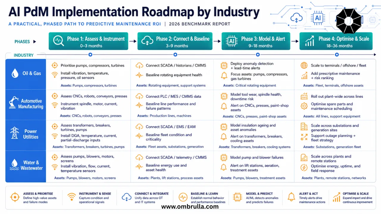
Oil & Gas / Petrochemicals

Priority Assets: Centrifugal pumps (crude, product, injection), gas compressors (centrifugal and reciprocating), rotating seals.

-
Start with high-consequence assets: Process-critical pumps and compressors where failure causes safety incidents or production shutdowns take priority over utility equipment.
-
Integrate with Process Safety Management (PSM) systems: AI PdM alerts should feed into HSE risk registers and permit-to-work workflows, not operate as standalone tools.
-
Explosion-proof sensor selection: ATEX Zone 1/2 (EU) or Class I Division 1/2 (US) certified sensors are mandatory - this constraint significantly narrows viable hardware options.
-
Oil analysis as foundation: Lubrication condition monitoring should be the first AI PdM layer deployed given the availability of existing oil sampling infrastructure at most refineries.

Automotive Manufacturing

Priority Assets: CNC machining centres (engine blocks, transmission components), transfer lines, compressed air systems, coolant pumps.

-
Integrate with OEE systems: AI PdM alerts should directly inform OEE calculations and feed into the daily operations meeting rhythm - positioning predictive maintenance as a production KPI, not a maintenance task.
-
Tool life management integration: Connect CNC AI PdM with the MES/ERP tool management module to automate tool replacement work orders based on AI wear signals rather than fixed-cycle rules.
-
Multi-machine fleet learning: Automotive plants often have banks of identical CNC machines. Deploy AI models that learn from the fleet collectively while maintaining per-machine baselines - dramatically reducing training data requirements.
-
Coordinate with model change cycles: AI model retraining requirements should be planned around vehicle model changeover periods to avoid baseline disruption.

Power Generation and Utilities

Priority Assets: Power transformers (transmission and distribution), cooling water pumps, gas/steam turbines, HV switchgear.

-
Prioritise DGA for transmission transformers: For assets rated 100 MVA and above, online DGA monitoring with AI interpretation should be considered standard practice, not optional.
-
Align with grid reliability frameworks: AI PdM programmes for utilities should be designed to support NERC CIP (North America) or equivalent reliability standard compliance documentation.
-
Seasonal load profiling: Transformer AI models must incorporate seasonal load variation patterns to avoid load-increase alerts during peak demand periods.
-
Substations as deployment units: Rather than asset-by-asset deployment, utilities achieve faster ROI by deploying AI PdM across all monitored assets within a substation simultaneously, enabling cross-asset correlation analysis.

Water and Wastewater Utilities

Priority Assets: Submersible and horizontal split-case pumps, blowers (WWTP aeration), UV disinfection systems.

-
Budget-constrained deployment: Water utilities typically operate under tighter capex constraints than industrial manufacturers. Prioritise sensor-light approaches: MCSA (motor current signature analysis) provides significant diagnostic value at low sensor cost.
-
Regulatory compliance integration: AI PdM alerts for treatment assets should integrate with SCADA systems and regulatory compliance reporting workflows.
-
Pump efficiency as primary KPI: For water utilities where energy is the largest operational cost, hydraulic efficiency monitoring (pump curve deviation) often delivers faster ROI than fault detection alone.
-
Remote monitoring for distributed assets: Water networks have geographically distributed pump stations. Prioritise cloud-connected edge AI platforms that minimise on-site infrastructure requirements.

AI Predictive Maintenance Implementation Roadmap

A successful AI PdM program should move through four maturity stages: prove the value case, establish trusted data, operationalise AI alerts, and then scale with RUL and advanced analytics.

Stage 1: Business Case & Asset Selection

Timeline: Months 0–3
Purpose: Identify where AI PdM can deliver the highest operational and financial value.

Focus Area	Key Actions
Asset Criticality	Rank assets based on production impact, safety risk, environmental exposure, failure history, age, and operating conditions.
Baseline Value	Capture current downtime hours, maintenance cost, emergency repair cost, failure frequency, and production loss.
Pilot Selection	Select 5–15 assets across 2–3 asset types, preferably including at least one asset with known degradation history.
Instrumentation Review	Identify available SCADA, DCS, MES, PLC, CMMS, and sensor data. Define additional sensor requirements.

Gate 1 Output: Prioritised asset list, pilot scope, baseline ROI model, and sensor gap assessment.

Stage 2: Data Foundation & Connectivity

Timeline: Months 3–9
Purpose: Build a reliable, secure, and validated data pipeline for AI model development.

Focus Area	Key Actions
Sensor Deployment	Install required sensors, gateways, edge devices, and connectivity infrastructure.
System Integration	Connect asset data using OPC-UA, MQTT, Modbus, Kepware, SCADA, DCS, MES, or API-based integrations.
Cybersecurity	Apply secure industrial connectivity practices aligned with ISA/IEC 62443 principles.
Data Validation	Check completeness, timestamp accuracy, sampling frequency, calibration, and signal quality.
Baseline Collection	Collect 60–90 days of clean operating data before enabling advanced AI alerts.

Gate 2 Output: Validated real-time data pipeline, baseline asset behaviour, and AI-ready data environment.

Stage 3: AI Modelling, Alerts & Workflow Adoption

Timeline: Months 9–18
Purpose: Deploy AI models, generate meaningful alerts, and embed them into maintenance workflows.

Focus Area	Key Actions
Model Activation	Enable anomaly detection and condition monitoring models with conservative thresholds.
Alert Strategy	Start with high-confidence alerts to reduce false alarms and build user trust.
CMMS/EAM Integration	Convert validated alerts into work orders, inspections, or maintenance recommendations.
Feedback Loop	Record every alert outcome: confirmed issue, false alarm, missed failure, or no action required.
Model Tuning	Review alert performance monthly and refine thresholds, features, and model logic.
Gate 3 Output	Operational AI alerting workflow, documented alert outcomes, improved model confidence, and early ROI evidence.

Gate 3 Output: Operational AI alerting workflow, documented alert outcomes, improved model confidence, and early ROI evidence.

Stage 4: Optimisation, RUL & Enterprise Scaling

Timeline: Months 18–36+
Purpose: Move from pilot success to mature, scalable predictive maintenance.

Focus Area	Key Actions
RUL Prediction	Enable Remaining Useful Life models for assets with sufficient failure and degradation history.
Portfolio Scaling	Expand from pilot assets to full asset classes, sites, or business units.
Cost Optimisation	Standardise sensors, gateways, dashboards, and integration patterns to improve deployment economics.
Advanced Analytics	Add multi-asset correlation, energy optimisation, process efficiency, and risk-based maintenance planning.
Continuous Improvement	Regularly review model performance, business impact, user adoption, and maintenance outcomes.

Gate 4 Output: Scaled PdM program, measurable ROI, improved uptime, lower maintenance cost, and enterprise-level asset intelligence.

Roadmap Summary

Stage	Timeline	Primary Goal
1. Business Case & Asset Selection	0–3 months	Choose the right assets and define ROI baseline.
2. Data Foundation & Connectivity	3–9 months	Build clean, secure, AI-ready data pipelines.
3. AI Modelling & Workflow Adoption	9–18 months	Deploy alerts, tune models, and integrate with maintenance execution.
4. Optimisation & Scaling	18–36+ months	Scale across assets, activate RUL, and expand advanced analytics.

Ready to Benchmark Your Own Assets?

Download our AI PdM Asset Assessment Template, calculate your potential ROI with our interactive tool, or schedule a 30-minute benchmark review with our industrial AI specialist team.

Book Expert Review

Frequently Asked Questions

Evidence-based answers to critical questions about AI PdM implementation, ROI, failure detection, and operational success.

Q1: What is a realistic payback period for industrial AI predictive maintenance?

Based on benchmark data from 2024–2026 deployments, payback periods range from 3–10 months for pump and compressor applications to 6–24 months for CNC and transformer deployments. The wide range reflects differences in asset criticality, production rates and how comprehensively the organisation captures all value streams (not just direct maintenance savings). Organisations that integrate AI PdM with production scheduling, energy management and supply chain (for parts pre-staging) achieve the fastest paybacks.

Q2: Which failure modes does AI PdM reliably detect, and which does it miss?

AI PdM is highly reliable for progressive, sensor-observable degradation: bearing wear, insulation ageing, impeller erosion, valve fatigue and oil contamination. It is substantially less reliable for sudden, low-precursor failures: fatigue fractures caused by material defects, failures caused by external impact or contamination events, and failure modes that occur below the detection frequency range of installed sensors. A well-designed AI PdM programme explicitly documents which failure modes are and are not covered — this is as important as the coverage itself.

Q3: How much training data does an AI PdM model require?

This depends on the algorithm type. Unsupervised anomaly detection models (which learn normal behaviour) can provide value after 60–90 days of clean baseline data. Supervised fault classification and RUL models require historical failure data — typically a minimum of 5–15 recorded failure events per failure mode before model accuracy is operationally acceptable. For assets with low failure frequency (e.g. large transformers), physics-informed AI models that embed domain knowledge to reduce training data dependency are strongly preferred.

Q4: What is a realistic false alarm rate to target?

Based on our benchmark data, a mature AI PdM system (18+ months operational) should target a false positive rate of 3–8% across all alert types. At initial deployment (0–6 months), rates of 15–40% are normal and should be expected and communicated to maintenance teams. Setting a 6-month 'alarm tuning' expectation upfront prevents the most common cause of early programme failure: team disengagement due to unrealistic early-stage expectations.

Q5: How accurate are RUL (Remaining Useful Life) predictions?

At a 30-day prediction horizon, best-in-class systems achieve 12–25% MAPE (Mean Absolute Percentage Error) under controlled conditions. In real-world deployments with variable load conditions and sensor data quality issues, MAPE typically increases to 20–40% at 30 days and 30–55% at 90 days. RUL predictions are most valuable as relative risk indicators and maintenance prioritisation tools rather than precise countdowns. Communicating this distinction to operations and planning teams is essential for sustained programme value.

Q6: Should we start AI PdM with cloud-based or edge-based processing?

The decision depends on three factors: data latency requirements, connectivity reliability and data sovereignty constraints. For assets where alerts require sub-second response (CNC tool breakage detection), edge processing is essential. For assets where hours of latency are acceptable (transformer DGA trending), cloud processing offers lower infrastructure cost and easier scaling. Most mature deployments in 2026 use a hybrid architecture: edge pre-processing for data reduction and real-time alerting, cloud models for complex pattern recognition and fleet-level analytics.

Q7: How do we ensure cybersecurity in an AI PdM deployment?

Follow IEC 62443 (Industrial Automation and Control Systems Security) as the baseline framework. Key controls include: network segmentation between OT sensor networks and IT/cloud infrastructure (never direct internet connectivity for sensors), encrypted data transmission (TLS 1.2 minimum), role-based access control for the AI platform, and third-party penetration testing of the sensor-to-cloud data path before go-live. Vendor security certification (SOC 2 Type II for cloud platforms, ISASecure certification for edge hardware) should be contractually required.

Q8: How do we measure whether our AI PdM programme is delivering value?

Establish a balanced KPI dashboard covering: (1) Technical metrics — alert precision (true positive rate), recall (sensitivity), false positive rate, lead time per confirmed fault; (2) Operational metrics — planned vs. unplanned maintenance ratio, mean time between failures (MTBF), OEE or availability; (3) Financial metrics — maintenance cost per asset, downtime hours avoided, parts spend vs. budget. Benchmark these metrics quarterly against pre-deployment baselines and industry benchmarks. Without a structured measurement framework, AI PdM value remains anecdotal and programmes lose organisational support at renewal time.

Conclusion

Industrial AI predictive maintenance in 2026 is a mature, proven discipline - but one that still demands precision in deployment, realism in expectations and rigour in measurement. The benchmark data in this report confirms that the value is real and substantial: maintenance cost reductions of 20–45%, alert lead times of days to months (depending on asset and failure mode), and ROI that routinely exceeds 400% over a five-year horizon when all value streams are captured.

But the same data underscores the importance of implementation quality. Systems deployed without adequate baseline data, proper contextual modelling and feedback-driven tuning consistently underperform. RUL predictions overstated as precise countdowns rather than probabilistic risk indicators erode trust. False alarm management, the unglamorous operational discipline that determines whether maintenance teams act on AI insights, often proves the difference between programme success and quiet abandonment.

The organisations that will derive the greatest competitive advantage from AI PdM in the next three years are those that invest not just in sensors and algorithms, but in the operational processes, data governance and human capability that allow AI insights to translate into maintenance decisions and, ultimately, into asset performance outcomes.